U0.L1 — PyTorch from Zero

Flow-Based Generative Models · UFRJ · 2026.2

01Environment sanity

Today you build the most-reused artifact of the course

By the end of these 90 minutes, every one of you owns a runnable, seeded, GPU-aware training loop template — under version control.

Everything trained later — flows, FFJORD, CFM, DDPM — is a filling of this template.

Lab format (this sets the standard for all labs):

• Scaffolded notebook with numbered TODOs; I live-code the first instance of each pattern, you complete the rest.
• Checkpoint cells every ~15 min: if the assert passes, continue. Nobody silently derails.
• Solutions released after the session.

One minute on the framing, then straight to the terminal. Every notebook part opens with a “reused in:” header — point at the first one when it appears.

Cell 0: does your machine work?

Reused in: every lab — this cell is the top of every notebook this course.

import random, numpy as np, torch

print(torch.__version__)
print("CUDA:", torch.cuda.is_available())

def set_seed(seed: int) -> None:
    random.seed(seed)
    np.random.seed(seed)
    torch.manual_seed(seed)
    torch.cuda.manual_seed_all(seed)

set_seed(0)
device = "cuda" if torch.cuda.is_available() else "cpu"

• set_seed is introduced now and used forever — three RNGs, one call.
• No GPU today is fine: everything in U0 runs on CPU. The code is written device-agnostic from day one.

Repo layout, fixed today

One convention for the whole course:

your-course-repo/
  labs/     # one notebook per lab session
  common/   # shared code -- today's template lives here
  runs/     # checkpoints, logs (gitignored)

common/train.py — the file we build in the training-loop block — is imported by every later lab. U0.L2 adds to it; nothing ever rewrites it.

30 seconds. The point is that common/ is a package, not a scratchpad.

02Tensors and broadcasting

Why we spend 20 minutes on shapes

Reused in: everywhere — broadcasting bugs are the #1 silent killer in generative-model code.

A shape bug in PyTorch usually does not crash. It broadcasts, produces a tensor of the wrong shape with plausible values, and trains to convergence on the wrong loss.

Our defense, from day one:

1. Know the broadcasting rules precisely — they are two sentences.
2. Assert shapes at boundaries (the checkpoint cells do this today; you do it in your own code tomorrow).

A tensor is data + three attributes

x = torch.randn(4, 3)          # shape (4, 3)
x.shape, x.dtype, x.device
# (torch.Size([4, 3]), torch.float32, device('cpu'))

The trio shape / dtype / device answers 90% of debugging questions.

• dtype: float32 is the default and the workhorse; float64 appears today only inside the autograd block’s gradient check.
• device: where the data lives. Operations require all operands on the same device — the rule we exercise at the end of this block.

view vs reshape vs permute

• view: reinterprets the same memory — never copies, fails if the layout is incompatible.
• reshape: view when possible, silent copy when not.
• permute (and .t()): reorders strides, not memory — the result is usually non-contiguous.

x = torch.arange(6).reshape(2, 3)
x.t().view(-1)        # RuntimeError: not contiguous
x.t().reshape(-1)     # works (silently copies)

The notebook’s tensors part plants one permute-then-view trap for you (TODO B.1). Read the error, understand why, then fix it.

Broadcasting: the two rules

To combine two tensors elementwise:

1. Align shapes from the right. Missing leading dimensions count as 1.
2. Two aligned dimensions are compatible iff they are equal or one of them is 1; size-1 dimensions are stretched (no copy) to match.

(4, 3) + (3,)    -> (4, 3)     # rule 1: (3,) reads as (1, 3)
(4, 1) + (1, 3)  -> (4, 3)     # rule 2: both stretch
(4, 3) + (4,)    -> error      # 3 vs 4: incompatible

That third line is the useful one: broadcasting fails loudly only when no dimension matches. The dangerous cases are the ones that succeed.

Worked exercise: pairwise squared distances

TODO B.2 (tensors part) — no loops allowed. For \(X \in \mathbb{R}^{n \times d}\), \(Y \in \mathbb{R}^{m \times d}\), compute the \((n, m)\) matrix \(D_{ij} = \lVert x_i - y_j \rVert^2\).

diff = X[:, None, :] - Y[None, :, :]   # -> (n, m, d)
D = diff.pow(2).sum(dim=-1)            # -> (n, m)

Checkpoint B:

assert torch.allclose(D, torch.cdist(X, Y) ** 2, atol=1e-5)

None-indexing inserts the size-1 dimensions; the broadcast does the double loop for you, vectorized.

Why this drill matters later

The shape discipline (batch, d) vs (batch, 1) vs (batch,) is exactly what makes the course’s losses implementable.

In U3.L1 you will meet losses of the form \[ \mathbb{E}_{t,\, x_1,\, x_0}\!\left[\, \big\lVert u_t^\theta(x_t) - (x_1 - x_0) \big\rVert^2 \,\right] \] where time \(t\) is a (batch,) tensor broadcast against (batch, d) states — one \(t\) per sample, stretched across \(d\) coordinates.

Course convention, fixed today: in every network signature, t is a (B,) float tensor with values in \([0,1]\). Today’s X[:, None, :] is that line of code, practiced early.

Name-drop only — do not explain the loss. The point is: this notation on the board IS the broadcasting exercise they just did.

Devices: one rule, one planted error

The rule: everything that touches in an operation lives on the same device. Model and data — you move both, explicitly.

model = model.to(device)
x, y = x.to(device), y.to(device)

TODO B.3 (tensors part) plants this error for you to read:

RuntimeError: Expected all tensors to be on the same device,
but found at least two devices, cuda:0 and cpu!

Diagnosis ritual: print .device of every operand, find the one that never got moved. It is the data loader’s output, roughly always.

03Autograd mechanics

Last session’s theory, today’s API

Reused in: U1.L1 (log-det checks), U2 (the adjoint discussion assumes you know what autograd stores), every lab.

In U0.T1 we proved: reverse-mode differentiation is right-to-left accumulation of VJPs along the computational graph, one cached activation per node.

Today you meet the same object as an API:

• requires_grad=True — “record operations on this tensor.”
• The graph is built on the fly, during the forward pass.
• .backward() — run the cotangent sweep; results land in .grad.

x = torch.tensor(2.0, requires_grad=True)
loss = x ** 2
loss.backward()
x.grad            # tensor(4.)

The accumulation bug, demonstrated live

.grad accumulates — backward() adds into it, never overwrites:

x = torch.tensor(2.0, requires_grad=True)
(x ** 2).backward(); print(x.grad)   # tensor(4.)
(x ** 2).backward(); print(x.grad)   # tensor(8.) <- summed!

• This is a feature (gradient accumulation over micro-batches, multi-head losses) with a default that bites beginners.
• This is why zero_grad() exists — and why it is a mandatory step of the canonical training loop, not an optional flourish.

The notebook’s autograd part (TODO C.1) hands you a training loop with the zero_grad() line deleted. Predict what the loss curve does, then run it.

Switching the tape off: no_grad and detach

with torch.no_grad():      # block-level: no graph built
    val_loss = loss_fn(model(x_val), y_val)

y = x.detach()             # tensor-level: cut from graph

• Evaluation must run under no_grad(): no graph \(\to\) no activation caching \(\to\) less memory, faster. Baked into the template’s evaluate().
• detach returns later (EMA weights, target networks). Today: know it exists and what it severs.

Rule of thumb: if no .backward() will ever be called on it, it should not be building a graph.

The gradient check: our independent witness

Autograd is code, and code is doubted. The course-wide ritual — the gradient-check — compares it against finite differences:

\[ \big[\nabla f(x)\big]_i \;\approx\; \frac{f(x + \varepsilon e_i) - f(x - \varepsilon e_i)}{2\varepsilon}, \qquad \text{error } O(\varepsilon^2). \]

No calculus, no tape — nothing shared with autograd. That independence is what makes it a witness.

TODO C.2 (autograd part): implement the witness

def finite_diff_grad(f, x, eps=1e-6):
    g = torch.zeros_like(x)
    for i in range(x.numel()):
        e = torch.zeros_like(x).view(-1)
        e[i] = eps
        e = e.view_as(x)
        g.view(-1)[i] = (f(x + e) - f(x - e)) / (2 * eps)
    return g

\(O(\text{numel})\) forward passes — a witness, never a training method. (The cost table in U0.T1 said exactly this about forward-mode columns.)

Checkpoint C: autograd vs. finite differences

The float64 trick — in float32, machine epsilon \(\approx 10^{-7}\) makes the FD quotient itself noisy; the check would fail even on correct gradients. Run the check in float64, train in float32.

mlp = mlp.double()                      # 3-layer MLP, float64
W = dict(mlp.named_parameters())["net.0.weight"]
g_ad = torch.autograd.grad(loss_fn(mlp(x), y), W)[0]
g_fd = finite_diff_grad(lambda w: loss_with(w), W)

rel = (g_ad - g_fd).abs().max() / (g_ad.abs().max() + 1e-12)
assert rel < 1e-4                       # Checkpoint C

“autograd computes exactly the VJP composition proved in U0.T1; finite differences is our independent witness. We will use autodiff-as-proof-assistant again in U1.L1 (log-det via jax.jacfwd).”

04nn.Module and optimizers

A model is a Module

Reused in: every model of the course.

class MLP(nn.Module):
    def __init__(self, d_in=2, d_h=64, d_out=2):
        super().__init__()
        self.net = nn.Sequential(
            nn.Linear(d_in, d_h), nn.SiLU(),
            nn.Linear(d_h, d_h), nn.SiLU(),
            nn.Linear(d_h, d_out),
        )
    def forward(self, x):
        return self.net(x)

What it buys: parameter registration (model.parameters()), device movement (model.to(device)), serialization — next slide.

state_dict: the model as data

torch.save(model.state_dict(), "runs/ckpt.pt")

model2 = MLP()
model2.load_state_dict(torch.load("runs/ckpt.pt"))

• A state_dict is a plain dict of name \(\to\) tensor. Portable, inspectable.
• Save the state dict, not the module object — pickled modules break across code versions; plain tensors do not.
• The template’s Checkpoint E asserts the round trip: save, load into a fresh model, verify every weight equal.

Optimizers: black boxes with a .step()

opt = torch.optim.SGD(model.parameters(), lr=1e-2)
opt = torch.optim.Adam(model.parameters(), lr=1e-3)

The API is three calls, and today that is all they are:

call	does
opt.zero_grad()	clear accumulated .grad (autograd block!)
loss.backward()	fill .grad via the VJP sweep
opt.step()	update parameters from .grad

Which optimizer, and why, is the next theory session’s topic (U0.T2). Today they are black boxes with a .step().

05The canonical training loop

The loop, live-coded once

Reused in: everything — this is the artifact.

for epoch in range(epochs):
    model.train()
    for x, y in train_loader:
        x, y = x.to(device), y.to(device)  # devices (tensors)
        loss = loss_fn(model(x), y)     # forward
        opt.zero_grad()                 # clear     (autograd)
        loss.backward()                 # VJP sweep (autograd)
        opt.step()                      # update    (optimizers)
    val_loss = evaluate(val_loader)     # no_grad   (autograd)

Five steps: forward \(\to\) loss \(\to\) zero_grad \(\to\) backward \(\to\) step. Every block of this lab reappears as one line of this loop — you have seen the whole lab converge to this slide.

The loop, animated

The artifact: training-loop-template

common/train.py
  set_seed(seed)
  class Trainer:
    __init__(model, opt, loss_fn, device, ckpt_dir, log_every)
    fit(train_loader, val_loader, epochs)
        # loop: forward -> loss -> zero_grad -> backward -> step
    evaluate(loader)                    # runs under no_grad
    save_ckpt(tag) / load_ckpt(tag)
  minimal CSV/stdout logger

Baked in from day one: seeding, device handling, checkpoint round-trip test, val evaluation under no_grad. MLflow integration arrives in U0.L2 — the logger stays minimal today.

This structure is binding: later labs import Trainer and fill it. Say that sentence verbatim.

The task: two moons

Deliberately the same dataset family that returns in U1.L1 (RealNVP), U2.L2 (FFJORD), U3.L1 (CFM) — you will watch four generations of models handle these two half-circles.

Today it is plain supervised classification: \(x \in \mathbb{R}^2\), \(y \in \{0, 1\}\), cross-entropy loss — the U0.T1 \(\widehat{R}_n(\theta) = \frac{1}{n} \sum_{i=1}^{n} \big(-\log \pi_{y_i}(x_i; \theta)\big)\), now as code:

loss_fn = nn.CrossEntropyLoss()   # takes LOGITS

Notebook TODOs E.1–E.4 (training-loop part): E.1 data + loaders, E.2 finish fit, E.3 evaluate, E.4 the checkpoint round trip. I live-code fit’s five-step core; you do the rest.

Checkpoint E: it trains

assert losses[-1] < 0.15 < losses[0]     # loss decreased
assert val_acc > 0.95                    # boundary is real

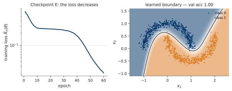
Plotting helper is given (plot_decision_boundary in the notebook) — today is not a matplotlib lab.

Watch it train

06Freeze and close

Freeze the template

Commit common/train.py now. Literally now — this is the lab’s last checkpoint:

git add common/train.py
git commit -m "training-loop-template v1"

• U0.L2 imports this exact file and adds hygiene: logging, schedules, checkpoint discipline. Nothing gets rewritten.
• If your template diverges from the contract slide, later lab scaffolds will not import cleanly. The contract is the interface.

Homework-lite, and what’s next

Homework-lite (unmarked, ~10 min): re-run the two-moons training with seeds 0, 1, 2. Look at the three final val accuracies. Eyeball the variance — no statistics required, just notice it is not zero.

That spread is the next session’s opening question (U0.T2).

• Next session (U0.T2): making training work — optimizers (the black boxes get opened), learning-rate schedules, initialization, normalization.
• Then (U0.L2): the hygiene stack — your template grows logging, schedules, and reproducibility discipline.

Bring the committed template to both.