U0.L1 — PyTorch from Zero
Session U0.L1 · date: see calendar-map
This is the first lab, and it produces the single most-reused artifact of the course: training-loop-template, a runnable, seeded, GPU-aware training loop under version control in your own repository. Everything trained later — normalizing flows, FFJORD, conditional flow matching, DDPM — is a filling of this template. The lab is deliberately, ruthlessly mechanical: no generative modeling, no optimizer theory (that is U0.T2), no training-hygiene depth (that is U0.L2). Today we make the machinery exist.
Lab format, which sets the standard for all labs in this course. You work in a scaffolded notebook (lab-u0l1.ipynb) with numbered TODOs; the instructor live-codes the first instance of each pattern, and you complete the rest. Checkpoint cells appear every ~15 minutes — if the assert passes, continue — so nobody silently derails. Solutions are released after the session. Each notebook part opens with a one-line “reused in:” header saying where in the course that part returns; the headers are reproduced in these notes.
Standing reference for the deep-learning mechanics in this lab: the relevant chapters of Bishop and Bishop (Bishop and Bishop 2024). The official PyTorch tutorials are a fine second pass after the lab.
A · Environment sanity
Reused in: every lab — Cell 0 is the top of every notebook in this course.
The first cell of every notebook this semester does three jobs: prove the environment works, fix the device, and seed every random number generator in sight.
import random

import numpy as np
import torch

print(torch.__version__)
print("CUDA available:", torch.cuda.is_available())


def set_seed(seed: int) -> None:
    """Seed all three RNG streams (python, numpy, torch incl. CUDA)."""
    random.seed(seed)
    np.random.seed(seed)
    torch.manual_seed(seed)
    torch.cuda.manual_seed_all(seed)


set_seed(0)
device = "cuda" if torch.cuda.is_available() else "cpu"
print("device:", device)
Two remarks. First, set_seed is introduced now and used forever: Python’s random, NumPy, and PyTorch keep independent RNG streams, and seeding only one of them is the classic way to produce a run that is “seeded” and still not reproducible. Second, no GPU today is fine — everything in U0 runs comfortably on CPU, and the code is written device-agnostic from day one, so nothing changes when a GPU appears later.
Repository layout, fixed today. One convention for the whole course:
your-course-repo/
  labs/     # one notebook per lab session
  common/   # shared course code -- today's template lives here
  runs/     # checkpoints, logs (gitignored)
common/ is a package, not a scratchpad: the file we build in Section 5 is imported by every later lab. U0.L2 adds to it; nothing ever rewrites it.
B · Tensors and broadcasting
Reused in: everywhere — broadcasting bugs are the #1 silent killer in generative-model code.
A shape bug in PyTorch usually does not crash. It broadcasts, produces a tensor of a plausible-looking shape with plausible-looking values, and trains to convergence on the wrong loss. This is why the lab spends twenty minutes on material that looks trivial: the broadcasting rules are two sentences, and knowing them precisely — rather than approximately — is the cheapest bug insurance this course sells.
The three attributes
A tensor is data plus three attributes, and the trio answers most debugging questions:
x = torch.randn(4, 3)
x.shape, x.dtype, x.device
# (torch.Size([4, 3]), torch.float32, device(type='cpu'))dtype.float32is the default and the workhorse.float64appears today in exactly one place — inside the gradient check of Section 3, where the extra precision is load-bearing. Integer tensors (int64) appear as class labels.device. Where the data lives. Operations require all operands on the same device; we exercise the failure mode at the end of this section.
view, reshape, permute — and the trap
viewreinterprets the same memory with a new shape. It never copies — and therefore fails when the requested shape is incompatible with the memory layout.reshapeisviewwhen possible and a silent copy when not.permute(and its two-dimensional shorthand.t()) reorders strides, not memory: the result views the same storage in a different order and is usually non-contiguous.
The composition of the last two facts is the trap planted in TODO B.1 (the notebook’s tensors part):
x = torch.arange(6).reshape(2, 3)
x.t().view(-1)       # RuntimeError: view size is not compatible ...
x.t().reshape(-1)    # works (silently copies): tensor([0, 3, 1, 4, 2, 5])
x.t().contiguous().view(-1)   # works, explicit about the copy
Read the error before fixing it. view refuses because after permute the elements are no longer laid out in the order the new shape requires; reshape shrugs and copies. Preferring reshape everywhere is a defensible style — but then the copies are invisible, which is exactly why it is worth once seeing the error view gives you.
Broadcasting: the two rules
To combine two tensors elementwise:
- Align shapes from the right. Missing leading dimensions count as size 1.
- Two aligned dimensions are compatible iff they are equal or one of them is 1; size-1 dimensions are stretched (without copying) to the other’s size.
(4, 3) + (3,)    -> (4, 3)   # rule 1: (3,) reads as (1, 3)
(4, 1) + (1, 3)  -> (4, 3)   # rule 2: both stretch
(4, 3) + (4,)    -> error    # aligned right: 3 vs 4, incompatible
The third line is the pedagogically valuable one: broadcasting fails loudly only when no dimension matches. The dangerous cases are the ones that succeed — (4, 3) + (1, 3) when you meant to add per-row, (n,) * (n, 1) producing an \((n, n)\) matrix out of two vectors. When in doubt, write the aligned shapes in a comment and assert the result’s shape.
Worked exercise: pairwise squared distances
TODO B.2 (tensors part) — no loops allowed. Given \(X \in \mathbb{R}^{n \times d}\) and \(Y \in \mathbb{R}^{m \times d}\), compute the \((n, m)\) matrix \(D_{ij} = \lVert x_i - y_j \rVert^2\).
None-indexing inserts the size-1 dimensions, and the broadcast performs the double loop, vectorized:
diff = X[:, None, :] - Y[None, :, :]   # (n,1,d) - (1,m,d) -> (n,m,d)
D = diff.pow(2).sum(dim=-1)            # (n, m)
Checkpoint B — the independent witness is the library:
assert torch.allclose(D, torch.cdist(X, Y) ** 2, atol=1e-5)(For large \(n, m, d\) the expansion \(\lVert x \rVert^2 - 2\,x^\top y + \lVert y \rVert^2\) is cheaper in memory than materializing the \((n, m, d)\) difference tensor — worth knowing, not required today.)
Why this drill matters later
The shape discipline (batch, d) vs (batch, 1) vs (batch,) is exactly what makes this course’s losses implementable. In U3.L1 you will meet losses of the form \[
\mathbb{E}_{t,\, x_1,\, x_0}\!\left[\,
\big\lVert u_t^\theta(x_t) - (x_1 - x_0) \big\rVert^2 \,\right],
\] where the time variable \(t\) is sampled per-example: in code, t is a (batch,) tensor broadcast against (batch, d) states — one \(t\) per sample, stretched across the \(d\) coordinates by exactly rule 1 above. The course-wide code convention is fixed today: in every network signature, t is a (B,) float tensor with values in \([0, 1]\). Today’s X[:, None, :] is that convention, practiced early. (What the loss means is U3’s business; today only its shape concerns us.)
Devices: one rule, one planted error
The rule: everything that touches in an operation lives on the same device — model and data, and you move both, explicitly:
model = model.to(device)
x, y = x.to(device), y.to(device)
TODO B.3 (tensors part) plants the canonical failure for you to read:
RuntimeError: Expected all tensors to be on the same device,
but found at least two devices, cuda:0 and cpu!
The diagnosis ritual: print .device of every operand in the failing line and find the one that never got moved. It is the data-loader output, roughly always — the model was moved once at construction, but the batches are born on CPU forever and must be moved inside the loop. This is precisely why the training-loop template of Section 5 has its .to(device) calls inside fit, not outside.
C · Autograd mechanics
Reused in: U1.L1 (log-det checks), U2 (the adjoint discussion assumes you know what autograd stores), every lab.
In the previous session (U0.T1) we proved that reverse-mode differentiation is right-to-left accumulation of VJPs along the computational graph, one cached activation per node (Proposition 1, U0.T1 — the artifact vjp-composition-proof). Today you meet the same object as an API.
The tape
requires_grad=Truemarks a tensor as “record operations on me.”- The computational graph is built on the fly during the forward pass — PyTorch is a define-by-run framework; the graph is whatever your Python code did this time.
.backward()runs the cotangent sweep; results accumulate in the.gradfields of the leaves.
x = torch.tensor(2.0, requires_grad=True)
loss = x ** 2
loss.backward()
x.grad          # tensor(4.)
The accumulation bug, demonstrated live
.grad accumulates: backward() adds into it, never overwrites.
x = torch.tensor(2.0, requires_grad=True)
(x ** 2).backward(); print(x.grad)   # tensor(4.)
(x ** 2).backward(); print(x.grad)   # tensor(8.)  <- accumulated!
Accumulation is a feature — it is how gradient accumulation over micro-batches and multi-term losses are implemented — with a default that bites beginners. This is why zero_grad() exists, and why it is a mandatory step of the canonical training loop, not an optional flourish. TODO C.1 (autograd part) hands you a training loop with the zero_grad() line deleted: predict what the loss curve does before running it. (It does not diverge immediately — stale gradients are momentum-like at first, which is what makes the bug so quiet.)
Switching the tape off
with torch.no_grad():          # block-level: no graph is built at all
    val_loss = loss_fn(model(x_val), y_val)

y = x.detach()                 # tensor-level: y shares data, exits the graph
Evaluation must run under no_grad(): with no backward pass coming, building the graph is pure waste — memory for cached activations, time for bookkeeping. The template’s evaluate() bakes this in. detach is the surgical version — it severs one tensor from the graph — and returns later in the course (EMA weights, target networks); today you only need to know what it severs.
Rule of thumb: if no .backward() will ever be called on it, it should not be building a graph.
The gradient check: finite differences as independent witness
Autograd is code, and code is doubted. The course-wide ritual — performed today for the first time and recurring course-wide — checks it against the one gradient estimator that involves no calculus and no tape: finite differences.
\[ \big[\nabla f(x)\big]_i \;\approx\; \frac{f(x + \varepsilon e_i) - f(x - \varepsilon e_i)}{2\varepsilon}, \qquad \text{central differences, error } O(\varepsilon^2). \]
TODO C.2 (autograd part) implements it, one coordinate at a time:
def finite_diff_grad(f, x: torch.Tensor, eps: float = 1e-6) -> torch.Tensor:
    """Central-difference gradient of scalar f at x, coordinate by coordinate."""
    g = torch.zeros_like(x)
    flat = g.view(-1)
    for i in range(x.numel()):
        e = torch.zeros_like(x).view(-1)
        e[i] = eps
        e = e.view_as(x)
        flat[i] = (f(x + e) - f(x - e)) / (2 * eps)
    return g
This costs \(O(\mathrm{numel}(x))\) forward passes — it is a witness, never a training method. The cost table in U0.T1 said exactly this about the forward-mode column: one pass per input direction. Finite differences is forward mode without even the accuracy.
The float64 trick. In float32, machine epsilon is \(\approx 1.2 \times 10^{-7}\): the subtraction in the difference quotient cancels catastrophically, and the check would fail even on perfectly correct gradients. The fix is to run the check in float64 (train in float32 as always): with machine epsilon \(\approx 2.2 \times 10^{-16}\), a step size near \(\varepsilon \approx 10^{-6}\) leaves both the truncation error (\(O(\varepsilon^2)\)) and the rounding error comfortably below the tolerance. This trick — temporarily promote precision to make a numerical test meaningful — recurs in U1.L1’s log-det checks.
Checkpoint C — autograd on a 3-layer MLP loss, against the witness, on a chosen weight tensor:
mlp = mlp.double()
x, y = x.double(), y
W = dict(mlp.named_parameters())["net.0.weight"]

g_ad = torch.autograd.grad(loss_fn(mlp(x), y), W)[0]
g_fd = finite_diff_grad(loss_as_function_of(W), W)

rel = (g_ad - g_fd).abs().max() / (g_ad.abs().max() + 1e-12)
assert rel < 1e-4
The callback, verbatim from the notebook:
“autograd computes exactly the VJP composition proved in U0.T1; finite differences is our independent witness. We will use autodiff-as-proof-assistant again in U1.L1 (log-det via
jax.jacfwd).”
D · nn.Module and optimizers
Reused in: every model of the course.
A model is a Module
import torch.nn as nn


class MLP(nn.Module):
    def __init__(self, d_in: int = 2, d_h: int = 64, d_out: int = 2):
        super().__init__()
        self.net = nn.Sequential(
            nn.Linear(d_in, d_h), nn.SiLU(),
            nn.Linear(d_h, d_h), nn.SiLU(),
            nn.Linear(d_h, d_out),
        )

    def forward(self, x: torch.Tensor) -> torch.Tensor:
        return self.net(x)
nn.Module buys three things: parameter registration — model.parameters() finds every weight recursively, which is what the optimizer consumes; device movement — model.to(device) moves all registered parameters at once; and serialization via state_dict. (SiLU rather than ReLU for continuity with the U-Nets and DiT blocks from U0.T4 onward; nothing today depends on the choice.)
state_dict: the model as data
torch.save(model.state_dict(), "runs/ckpt.pt")

model2 = MLP()
model2.load_state_dict(torch.load("runs/ckpt.pt"))
A state_dict is a plain dictionary of name → tensor: portable and inspectable. Save the state dict, not the module object — a pickled module silently breaks when the class definition changes; plain tensors do not. The template’s Checkpoint E asserts the full round trip: save, load into a freshly constructed model, verify every parameter equal.
Optimizers: black boxes with a .step()
opt = torch.optim.SGD(model.parameters(), lr=1e-2)
opt = torch.optim.Adam(model.parameters(), lr=1e-3)
The API is three calls:
| call | does |
|---|---|
opt.zero_grad() |
clear accumulated .grad (Section 3) |
loss.backward() |
fill .grad via the VJP sweep |
opt.step() |
update parameters in place from .grad |
Which optimizer and why is the next theory session’s topic (U0.T2); today they are black boxes with a .step(). We instantiate both, we use Adam for the lab task, and we resist all temptation to discuss momentum.
E · The canonical training loop → training-loop-template
Reused in: everything — this is the artifact.
The instructor live-codes the skeleton; notebook TODOs E.1–E.4 (training-loop part) complete it on the lab task — E.1 data + loaders, E.2 finish fit, E.3 evaluate under no_grad, E.4 the checkpoint round trip. The loop itself is five steps — forward → loss → zero_grad → backward → step — and every block of this lab reappears as one line of it:
for epoch in range(epochs):
    model.train()
    for x, y in train_loader:
        x, y = x.to(device), y.to(device)   # devices (tensors block)
        loss = loss_fn(model(x), y)         # forward
        opt.zero_grad()                     # clear (autograd block)
        loss.backward()                     # VJP sweep (autograd block)
        opt.step()                          # update (optimizers block)
    val_loss = evaluate(val_loader)         # no_grad (autograd block)
The loop as a state machine — what changes at each of the five steps (activations cached on forward, .grad cleared then filled, parameters moved on step). The same cycle returns with a different loss box in U1.L1, the U2 labs, and U3.L1:
The template contract
This structure is binding for all later labs — they import Trainer and fill it, so the interface is frozen today:
common/train.py
  set_seed(seed)
  class Trainer:
    __init__(model, opt, loss_fn, device, ckpt_dir, log_every)
    fit(train_loader, val_loader, epochs)
        # loop: forward -> loss -> zero_grad -> backward -> step
    evaluate(loader)                        # runs under no_grad
    save_ckpt(tag) / load_ckpt(tag)
  minimal CSV/stdout logger
Requirements baked in from day one: seeding (set_seed at the top of every run), device handling (batches moved inside fit, never assumed pre-moved), checkpoint save/load round-trip test (assert equal weights after reload), and val evaluation under no_grad. The logger stays a minimal CSV/stdout affair on purpose: experiment-tracker integration (MLflow) happens in U0.L2, not today.
The task: two moons
The lab task is two-moons classification — deliberately the same dataset family that returns in U1.L1 (RealNVP learns to generate it), U2.L2 (FFJORD flows it), and U3.L1 (conditional flow matching transports noise onto it). You will watch four generations of models handle these two half-circles; today’s baseline is worth having.
Today it is plain supervised classification: \(x \in \mathbb{R}^2\), \(y \in \{0, 1\}\), and the loss is the U0.T1 cross-entropy, \[ \widehat{R}_n(\theta) \;=\; \frac{1}{n} \sum_{i=1}^{n} \big({-\log \pi_{y_i}(x_i;\theta)}\big), \] now as code:
loss_fn = nn.CrossEntropyLoss() # takes LOGITS, not probabilities(CrossEntropyLoss applies log_softmax internally — passing it probabilities is a classic silent bug; the numerically stable form is the fused one.)
A self-contained, seeded two-moons generator (also in the notebook, so there is no scikit-learn dependency):
def two_moons(n: int, noise: float = 0.08,
              generator: torch.Generator | None = None):
    """n points on two interleaved half-circles, labels in {0, 1}."""
    half = n // 2
    t0 = torch.rand(half, generator=generator) * torch.pi
    t1 = torch.rand(n - half, generator=generator) * torch.pi
    x0 = torch.stack([torch.cos(t0), torch.sin(t0)], dim=1)
    x1 = torch.stack([1.0 - torch.cos(t1), 0.5 - torch.sin(t1)], dim=1)
    x = torch.cat([x0, x1]) + noise * torch.randn(n, 2, generator=generator)
    y = torch.cat([torch.zeros(half), torch.ones(n - half)]).long()
    return x, y
Checkpoint E: it trains
Two asserts close the block — the loss decreases, and the boundary is real:
assert losses[-1] < 0.15 < losses[0]     # training loss decreased
assert val_acc > 0.95                    # >95% val accuracy on two moons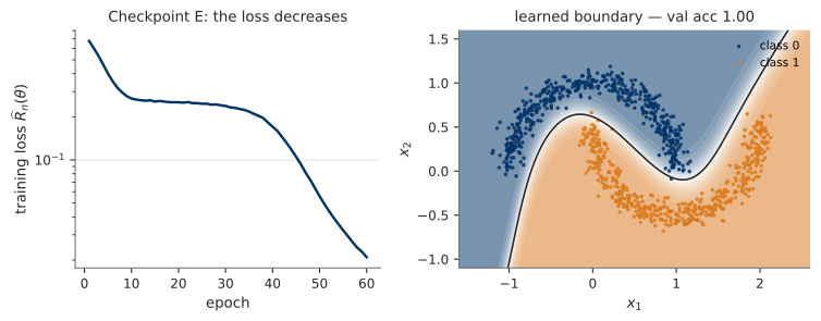
scripts/python/fig_u0_l1_two_moons.py).The plotting helper (plot_decision_boundary) is given in the notebook — today is not a matplotlib lab. It evaluates the trained network on a grid (under no_grad, of course) and shades the class-1 probability.
The trajectory is worth watching once: the boundary starts near-linear, sits through the loss plateau as a straight cut, and carves the interleaved region exactly as the plateau breaks (epochs ~40–55 in this seed-0 reference run):
F · Freeze and close
Commit common/train.py now — this is the lab’s final checkpoint:
git add common/train.py && git commit -m "training-loop-template v1"U0.L2 imports this exact file and adds the hygiene stack — logging, schedules, checkpoint discipline; nothing gets rewritten. If your template diverges from the contract box above, later lab scaffolds will not import cleanly: the contract is the interface.
Homework-lite (unmarked, ~10 minutes). Re-run the two-moons training with seeds 0, 1, and 2, and look at the three final validation accuracies. Eyeball the variance — no statistics required, just notice that it is not zero. That spread — where it comes from, when it matters, and how to report it honestly — is the next session’s opening question (U0.T2).
Next. U0.T2: making training work — the optimizer black boxes get opened, plus learning-rate schedules, initialization, and normalization. Then U0.L2: the hygiene stack — your template grows logging, schedules, and reproducibility discipline.