U0.T3 — Latent Variables and the VAE

Session U0.T3 · date: see calendar-map

Slides Slides PDF

This is the first genuinely generative session of the course. Until now we fit a function \(f_\theta \colon x \mapsto y\) and judged it by how well it predicted. From here on we fit a distribution \(p_\theta\) and judge it by how well it explains — and immediately run into the difficulty that organizes the next four months: for an expressive model, \(\log p_\theta(x)\) is easy to write down and hard to compute.

The session has three deliverables. First, the latent-variable frame and a precise account of why its marginal likelihood is intractable (Section 3). Second, the ELBO, derived twice, with the gap identity boxed as the artifact elbo-derivation (Section 4) — the box later sessions cite by name. Third, the reparameterization trick, presented as a general device for differentiating through sampling rather than a VAE-specific hack (Section 5). A 20-minute panorama of GANs and autoregressive models (Section 6) supplies the vocabulary you will need to read the literature, and nothing more.

Standing references for the unit: (Bishop and Bishop 2024; Murphy 2023). The primary sources for today’s objects are (Kingma and Welling 2014; Rezende, Mohamed, and Wierstra 2014) for the VAE and amortized variational inference, and (Goodfellow et al. 2014) for the panorama.

A notation collision, resolved once

The course reserves the unsubscripted letter \(q\) for the data distribution — the thing we are trying to model, with samples \(x \sim q\). The VAE literature independently uses \(q\) for the encoder, an approximation to a posterior. Two different objects, one letter, and both appear in every equation today.

• \(q\), unsubscripted, is always the data distribution on \(\mathbb{R}^{d}\).
• Variational / encoder distributions always carry their subscript: \(q_\varphi(z \mid x)\). There is no unsubscripted encoder anywhere in this course.
• The decoder is \(p_\theta(x \mid z)\), the prior over latents is \(p(z) = \mathcal{N}(0, I_{d_z})\), and \(\theta\), \(\varphi\) are the decoder and encoder parameters respectively.

This is recorded in the course symbol table (L1 §4) as a ruling, not a suggestion. It is worth thirty seconds of your attention for a reason beyond bookkeeping: notation hygiene is what lets us put diffusion and flow matching in the same equations later without silently changing what a symbol means. A course that is casual about \(q\) today will be unable to state the Rosetta Stone in U3.

One more symbol to reserve: \(\varepsilon \sim \mathcal{N}(0, I)\) will denote the auxiliary noise variable of Section 5. When \(\varepsilon_\theta\) reappears in U3’s diffusion detour it will be a network, not a random variable; the subscript again does the distinguishing work.

From fitting functions to fitting distributions

U0.T1 set up supervised learning twice: as empirical risk minimization, and as maximum likelihood. The maximum-likelihood view is the one that generalizes. Written for an unsupervised problem — no labels, just samples \(x \sim q\) — it reads

\[ \max_{\theta} \; \mathbb{E}_{x \sim q}\big[\log p_\theta(x)\big], \tag{1}\]

equivalently \(\min_\theta \mathrm{KL}(q \,\|\, p_\theta)\) up to a constant in \(\theta\). Nothing here is new. What is new is that the objective is no longer computable.

For a supervised model, \(\log p_\theta(y \mid x)\) was a closed-form expression in the network output — a squared error, a cross-entropy. For a generative model of images we want \(p_\theta\) to be expressive, and every construction that buys expressivity makes Equation 1 harder to evaluate. That tension is the subject of the whole course. U0.T1 planted the sentence; here it is again, because today is its first concrete instance:

“Much of this course is about what to do when the model’s likelihood is easy to sample but hard to evaluate — or vice versa.”

The VAE sits squarely on the “easy to sample, hard to evaluate” side. By the end of Section 6 you will have a three-way classification of generative models organized by exactly this axis.

Latent-variable models and the intractability loop

The modeling move

Build a complicated distribution out of simple parts by marginalizing a hidden variable:

Fix a prior \(p(z)\) on a latent space \(\mathbb{R}^{d_z}\) and a decoder (conditional likelihood) \(p_\theta(x \mid z)\) on \(\mathbb{R}^{d}\). The model distribution is the marginal \[ p_\theta(x) \;=\; \int p_\theta(x \mid z)\, p(z)\, \mathrm{d}z \;=\; \mathbb{E}_{z \sim p(z)}\big[p_\theta(x \mid z)\big]. \tag{2}\] Sampling is a two-step ancestral procedure: draw \(z \sim p(z)\), then \(x \sim p_\theta(x \mid z)\).

Throughout, \(p(z) = \mathcal{N}(0, I_{d_z})\) and \(p_\theta(x \mid z) = \mathcal{N}\big(x;\, g_\theta(z),\, \sigma^2 I_d\big)\) for a network \(g_\theta\) — each individual piece as simple as a distribution gets.

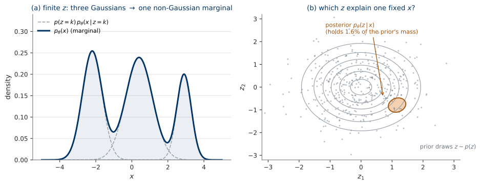
The expressivity does not come from the pieces. It comes from the marginalization. The finite version makes this visible with no machinery at all: let \(z\) take three values with probabilities \(p(z = k)\), so Equation 2 is a three-component mixture.

Figure 1: (a) A latent variable with three states. Each conditional \(p_\theta(x \mid z = k)\) is a Gaussian (dashed); the marginal \(p_\theta(x) = \sum_k p(z{=}k)\, p_\theta(x \mid z{=}k)\) (solid) is multimodal, and therefore not a Gaussian. (b) The same construction in continuous latent space, and the problem it creates. Gray contours and dots: the prior \(p(z)\) and \(400\) draws from it. Orange: the set of \(z\) that actually explain one fixed observation \(x\) — formally the posterior \(p_\theta(z \mid x)\), drawn at its \(95\%\) contour. That region holds \(1.6\%\) of the prior’s mass, so a draw from \(p(z)\) almost never lands in it.

Why Equation 2 cannot be computed

Equation 2 is an expectation, and expectations have an obvious estimator. Draw \(z_1, \dots, z_K \sim p(z)\) independently and take

\[ \widehat{p}_\theta(x) \;=\; \frac{1}{K} \sum_{k=1}^{K} p_\theta(x \mid z_k), \qquad \mathbb{E}_{z_{1:K} \sim p(z)}\big[\widehat{p}_\theta(x)\big] = p_\theta(x). \tag{3}\]

The estimator is unbiased. It is also useless, and the reason is Figure 1(b). For a fixed \(x\), the decoder \(p_\theta(x \mid z)\) is sharply peaked in \(z\): only latents that decode to something near \(x\) contribute, and those occupy a vanishing fraction of the prior’s mass. Almost every term in the sum Equation 3 is numerically zero, and the estimate is dominated by whether any draw happened to land in the good region.

This is not a rhetorical claim; it is measurable. Figure 2 runs Equation 3 on a deliberately tractable toy — a linear decoder \(g_\theta(z) = Az + b\), for which \(p_\theta(x) = \mathcal{N}(x;\, b,\, AA^\top + \sigma^2 I)\) is known exactly — and plots the error against the truth.

Figure 2: Median relative error of the importance-sampling estimator of \(p_\theta(x)\) against the number of samples \(K\), over \(400\) independent repetitions, on a linear-decoder toy where the exact value is available in closed form. Orange: proposal \(= p(z)\), the naive estimator Equation 3. Blue: a crude diagonal Gaussian near the true posterior — a stand-in for a trained encoder \(q_\varphi(z \mid x)\). At \(K = 100\) the naive estimator is still \(68\%\) wrong while the posterior-guided one is \(8\%\) wrong; the naive estimator’s flat stretch at \(100\%\) error is the regime where no draw has landed in the explaining region, so the estimate is essentially zero.

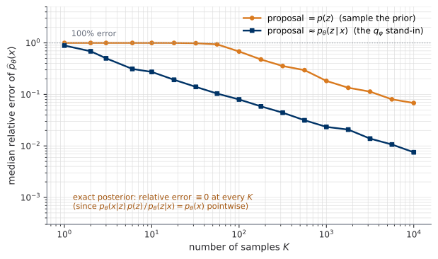
Two things deserve emphasis. First, the toy is linear precisely so that a ground truth exists to measure against; replace \(A z + b\) by a neural network and the reference line, the exact posterior, and the closed-form marginal all disappear at once. Second, an unbiased estimator with catastrophic variance is not a partial solution. Plugging Equation 3 into Equation 1 gives \(\log \widehat{p}_\theta(x)\), which is not even unbiased for \(\log p_\theta(x)\) — the logarithm of an unbiased estimator is biased downward by Jensen’s inequality, and by an amount that grows with the variance we just failed to control.

The object that would fix it, and why we cannot have it

Importance sampling says: sample from a proposal \(r(z)\) instead of the prior, and reweight.

\[ p_\theta(x) \;=\; \mathbb{E}_{z \sim r}\!\left[\frac{p_\theta(x \mid z)\, p(z)}{r(z)}\right]. \tag{4}\]

There is a proposal for which this is not merely low-variance but exact. Take \(r = p_\theta(\cdot \mid x)\), the true posterior. By Bayes’ rule \(p_\theta(z \mid x) = p_\theta(x \mid z)\, p(z) / p_\theta(x)\), so the ratio inside the expectation equals \(p_\theta(x)\) for every \(z\) — a random variable with zero variance. One sample would do.

So the posterior is exactly the object we want. And it is exactly the object we cannot have, because Bayes’ rule computes it from \(p_\theta(x)\), which is what we were trying to find.

Figure 3: The circular dependency that motivates everything after this section. Neither object can be computed first.

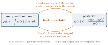
Intractable likelihoods are the recurring obstacle of this course, and different families answer it differently. U1’s answer is invertibility: build \(p_\theta\) from a bijection so that the change-of-variables formula gives \(\log p_\theta(x)\) exactly, with no marginalization at all. The VAE’s answer is bounding: give up on computing \(\log p_\theta(x)\) and optimize a tractable lower bound instead. Keep both strategies on your map — much of the course is a tour of such answers, and Flow Matching’s answer (U3) is a third one that avoids the likelihood entirely.

The ELBO

The plan: introduce an arbitrary distribution \(q_\varphi(z \mid x)\) over latents, obtain a computable lower bound on \(\log p_\theta(x)\), and then find out exactly what we gave up.

First derivation: Jensen

Insert \(q_\varphi\) into Equation 2, multiplying and dividing:

\[ \begin{aligned} \log p_\theta(x) &= \log \int p_\theta(x \mid z)\, p(z)\, \mathrm{d}z \\[2pt] &= \log \int q_\varphi(z \mid x)\, \frac{p_\theta(x \mid z)\, p(z)}{q_\varphi(z \mid x)}\, \mathrm{d}z \\[2pt] &= \log\, \mathbb{E}_{z \sim q_\varphi(\cdot \mid x)}\!\left[ \frac{p_\theta(x \mid z)\, p(z)}{q_\varphi(z \mid x)}\right] \\[2pt] &\;\ge\; \mathbb{E}_{z \sim q_\varphi(\cdot \mid x)}\!\left[ \log \frac{p_\theta(x \mid z)\, p(z)}{q_\varphi(z \mid x)}\right] \\[2pt] &= \underbrace{\mathbb{E}_{z \sim q_\varphi(\cdot \mid x)}\big[\log p_\theta(x \mid z)\big] - \mathrm{KL}\big(q_\varphi(z \mid x) \,\big\|\, p(z)\big)}_{\textstyle =: \; \mathrm{ELBO}(\theta, \varphi; x)} . \end{aligned} \tag{5}\]

The inequality is Jensen’s, applied to the concave \(\log\).¹ The name is now literal: the evidence lower bound, “evidence” being the classical term for the marginal likelihood \(p_\theta(x)\).

Both terms of Equation 5 are computable, which is the entire point: the first is an expectation we can estimate by sampling from \(q_\varphi\) (a distribution we designed, so we can sample it), and the second is a KL between two Gaussians, available in closed form.

The one fact about KL we need today

For distributions \(a, b\) with \(a \ll b\), \(\;\mathrm{KL}(a \,\|\, b) := \mathbb{E}_{y \sim a}\big[\log \tfrac{a(y)}{b(y)}\big] \ge 0\), with equality if and only if \(a = b\) almost everywhere.

Proof. Apply Jensen’s inequality to the concave \(\log\): \[ -\mathrm{KL}(a \,\|\, b) = \mathbb{E}_{y \sim a}\!\left[\log \frac{b(y)}{a(y)}\right] \;\le\; \log\, \mathbb{E}_{y \sim a}\!\left[\frac{b(y)}{a(y)}\right] = \log \int b(y)\, \mathrm{d}y = \log 1 = 0 . \] Strict concavity of \(\log\) makes the inequality strict unless \(b/a\) is \(a\)-almost-surely constant, which given that both integrate to one forces \(a = b\). \(\square\)

That is all we need. KL gets its full treatment in UP.A — including the Gaussian closed forms you will use in the next lab (U0.L3) as black boxes, and the sense in which it is not a distance (it is not symmetric and violates the triangle inequality). For the lab, the one closed form to have on hand is

\[ \mathrm{KL}\big(\mathcal{N}(\mu, \operatorname{diag}(\sigma^2)) \,\big\|\, \mathcal{N}(0, I_{d_z})\big) = \frac{1}{2} \sum_{j=1}^{d_z} \big(\mu_j^2 + \sigma_j^2 - 1 - 2\log \sigma_j\big), \tag{6}\]

quoted here without proof and derived in UP.A.

Second derivation: the gap identity

Jensen tells us \(\mathrm{ELBO} \le \log p_\theta(x)\). It does not tell us by how much. The second derivation does, and it is the session’s central result.

For every \(\theta\), every \(\varphi\), and every \(x\) with \(p_\theta(x) > 0\), \[ \log p_\theta(x) \;=\; \mathrm{ELBO}(\theta, \varphi; x) \;+\; \mathrm{KL}\big(q_\varphi(z \mid x) \,\big\|\, p_\theta(z \mid x)\big). \tag{7}\] The bound’s slack is exactly the KL divergence from the variational distribution to the true posterior — no more, no less.

Proof. Start from the KL on the right and substitute Bayes’ rule, \(p_\theta(z \mid x) = p_\theta(x \mid z)\, p(z) / p_\theta(x)\):

\[ \begin{aligned} \mathrm{KL}\big(q_\varphi(z \mid x) \,\big\|\, p_\theta(z \mid x)\big) &= \mathbb{E}_{z \sim q_\varphi(\cdot \mid x)}\big[\log q_\varphi(z \mid x) - \log p_\theta(z \mid x)\big] \\ &= \mathbb{E}_{z \sim q_\varphi(\cdot \mid x)}\big[\log q_\varphi(z \mid x) - \log p_\theta(x \mid z) \\ &\hphantom{{}={}} \qquad\quad - \log p(z) + \log p_\theta(x)\big] \\ &= -\,\mathbb{E}_{z \sim q_\varphi(\cdot \mid x)}\!\left[ \log \frac{p_\theta(x \mid z)\, p(z)}{q_\varphi(z \mid x)}\right] + \log p_\theta(x) \\ &= -\,\mathrm{ELBO}(\theta, \varphi; x) + \log p_\theta(x), \end{aligned} \]

where the third line uses that \(\log p_\theta(x)\) does not depend on \(z\), so it passes through the expectation unchanged, and the fourth line is the definition in Equation 5. Rearranging gives Equation 7. \(\square\)

Note what Equation 7 delivers for free: since KL \(\ge 0\), it re-proves \(\mathrm{ELBO} \le \log p_\theta(x)\) without invoking Jensen a second time. The two derivations are not redundant — the first shows the bound exists, the second identifies it.

Reading the identity in both directions

Equation 7 is worth reading out loud twice, because each direction is a different idea.

Direction 1 — hold \(\theta\) fixed and vary \(\varphi\). The left-hand side does not depend on \(\varphi\) at all. So maximizing the ELBO over \(\varphi\) cannot change \(\log p_\theta(x)\); it can only shrink the KL term. Optimizing the encoder is doing approximate posterior inference, and tightening the bound is the same operation as improving the posterior approximation. This is the whole of variational inference in one line.

Direction 2 — ask what the gap is. At any fixed \(\varphi\), the number we report is short of the truth by precisely the posterior mismatch. If \(q_\varphi\) is restricted to diagonal Gaussians and the true posterior is not one, that gap never closes, and every likelihood we report is an underestimate by an amount we cannot measure.

Figure 4: The gap identity as a picture. The total height \(\log p_\theta(x)\) is fixed — it does not depend on \(\varphi\) — so the only way the bound rises is by the gap shrinking.

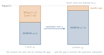
The animation below runs the ascent for real, on the linear-decoder toy of Figure 2, so every quantity in it is computed rather than drawn. Two details repay attention. The dashed ceiling never moves — that is the identity. And the ending is honest: gradient ascent drives \(\mu_\varphi\) to the true posterior mean exactly, but a diagonal \(q_\varphi\) cannot represent a correlated posterior, so \(0.013\) nats of gap survive. That residue is the floor for any diagonal family here, and it is a useful calibration: a numerically tiny KL can still mean a qualitatively wrong shape.

The habit to form here outlives the VAE: whenever this course gives you a bound, ask what the gap is. A bound whose slack is an identified quantity is a scientific object; a bound whose slack is unknown is a number that flatters you.

Anatomy: reconstruction against compression

Written as in Equation 5, the objective splits into two terms that pull in opposite directions:

\[ \mathrm{ELBO}(\theta, \varphi; x) = \underbrace{\mathbb{E}_{z \sim q_\varphi(\cdot \mid x)}\big[\log p_\theta(x \mid z)\big] }_{\text{reconstruction: decode } z \text{ back to } x} \;-\; \underbrace{\mathrm{KL}\big(q_\varphi(z \mid x) \,\big\|\, p(z)\big) }_{\text{regularization: keep } q_\varphi \text{ near the prior}} . \]

The reconstruction term is maximized by an encoder that packs as much information about \(x\) into \(z\) as possible — in the limit, a deterministic near-lookup. The KL term is minimized by an encoder that ignores \(x\) entirely and returns the prior, at which point the latent carries no information and reconstruction collapses. Training resolves the tug-of-war, and where it resolves is a property of the model and the data, not something we set directly.

Because the two terms behave so differently, the course convention is to log them separately, never only their sum (this is the “composite losses log their parts” rule from U0.T2’s recipe card). In the next session (U0.L3) you will look at the KL term broken down per latent dimension and see something specific in it.

Amortization: why this is an algorithm and not just an identity

Classical variational inference optimizes a separate \(q^{(i)}(z)\) for each datapoint \(x_i\) — an inner optimization loop per example, at training and at test time, with no way to handle an \(x\) it has not seen. The VAE’s contribution (Kingma and Welling 2014; Rezende, Mohamed, and Wierstra 2014) is to replace that per-datapoint optimization with a single network:

\[ x \;\longmapsto\; \big(\mu_\varphi(x),\, \sigma_\varphi(x)\big), \qquad q_\varphi(z \mid x) = \mathcal{N}\big(z;\, \mu_\varphi(x),\, \operatorname{diag}(\sigma_\varphi(x)^2)\big). \tag{8}\]

One forward pass produces the variational parameters for any \(x\), including one never seen in training. The cost of inference is amortized across the dataset. This is what turns Equation 7 from a fact about a single datapoint into a scalable training algorithm — and it is a pattern worth recognizing, because “replace a per-instance optimization by a network trained to predict its solution” is one of the field’s most reused moves.

The price is an extra source of slack: even the best diagonal-Gaussian \(q_\varphi\) for this \(x\) may be unreachable by this network, which is a second gap on top of the family restriction. It is called the amortization gap, and it is named here only so the term does not surprise you in a paper.

File this derivation pattern away: a variational bound plus Gaussian algebra returns in the D2 detour of U3, where the surprising punchline will be about the weighting of the resulting loss — not its minimizer. That is the whole flag; nothing more is claimed here, and you should resist the temptation to guess the rest.

Reparameterization: differentiating through sampling

The problem, stated precisely

Training needs \(\nabla_\varphi \mathrm{ELBO}(\theta, \varphi; x)\), and the reconstruction term has the shape

\[ \nabla_\varphi \, \mathbb{E}_{z \sim q_\varphi(\cdot \mid x)}\big[f(z)\big], \qquad f(z) = \log p_\theta(x \mid z). \tag{9}\]

Compare this with every gradient U0.T1 taught you to take. There, \(\varphi\) entered the integrand, and differentiation commuted with the expectation. Here \(\varphi\) indexes the distribution being sampled from; it does not appear in \(f\) at all. Writing the estimator \(\frac{1}{K}\sum_k f(z_k)\) and calling .backward() returns zero — correctly, since \(f\) genuinely does not depend on \(\varphi\). The sampling step is not a differentiable node; it is a discontinuous jump from a distribution to a draw.

The device

Move the parameter out of the sampling distribution and into the integrand, by a change of the sampling variable.

Let \(\varepsilon \sim \mathcal{N}(0, I_{d_z})\), a distribution carrying no parameters, and set \[ z \;=\; \mu_\varphi(x) + \sigma_\varphi(x) \odot \varepsilon , \tag{10}\] with \(\odot\) the elementwise product. Then \(z \sim \mathcal{N}\big(\mu_\varphi(x), \operatorname{diag}(\sigma_\varphi(x)^2)\big) = q_\varphi(z \mid x)\), so for any integrable \(f\), \[ \mathbb{E}_{z \sim q_\varphi(\cdot \mid x)}\big[f(z)\big] = \mathbb{E}_{\varepsilon \sim \mathcal{N}(0, I)}\big[ f\big(\mu_\varphi(x) + \sigma_\varphi(x) \odot \varepsilon\big)\big], \] and therefore \[ \nabla_\varphi \, \mathbb{E}_{z \sim q_\varphi(\cdot \mid x)}\big[f(z)\big] = \mathbb{E}_{\varepsilon \sim \mathcal{N}(0, I)}\big[ \nabla_\varphi\, f\big(\mu_\varphi(x) + \sigma_\varphi(x) \odot \varepsilon\big)\big]. \tag{11}\]

The exchange of \(\nabla_\varphi\) and \(\mathbb{E}\) in Equation 11 is now the ordinary one, because the measure being integrated against is \(\mathcal{N}(0, I)\) — fixed, independent of \(\varphi\). Everything \(\varphi\)-dependent has moved inside \(f\), where autodiff can reach it. The Monte Carlo estimator with a single \(\varepsilon\) per datapoint is unbiased and, in practice, low-variance enough to train with.

The framing to keep is the general one: reparameterize the sampling variable, then push the gradient inside. Nothing in Equation 10 is specific to the VAE; the construction works for any distribution expressible as a differentiable transform of a parameter-free base — location-scale families directly, and others through their inverse CDF or an accept-reject relaxation.

The autodiff view

Figure 5 is the same picture as U0.T1’s computational graph, with one node changed.

Figure 5: Left: \(\varphi\) parameterizes the distribution a random node is drawn from, so the reverse sweep of U0.T1 hits a node that is not a function of \(\varphi\) and stops. Right: reparameterized. The randomness enters as an external input \(\varepsilon\) whose law carries no parameter, \(z\) becomes an ordinary differentiable node, and the cotangent chain runs all the way back to \(\varphi\).

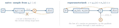
The computational graph now contains a random input. That is the entire conceptual shift, and it is why the trick is a graph-level statement rather than a probability-theory one: we have not changed the distribution of anything, only which quantities the graph treats as inputs.

The animation traces the reverse sweep itself — the same pulse U0.T1 used for reverse-mode autodiff, first dying at the sampling node, then reaching \(\varphi\) once the graph is rewritten:

The alternative, named but not developed

When a distribution admits no such reparameterization — discrete latents, most obviously — the general-purpose fallback is the score-function (or REINFORCE) estimator, which uses \(\nabla_\varphi q_\varphi = q_\varphi \nabla_\varphi \log q_\varphi\) to write

\[ \nabla_\varphi \, \mathbb{E}_{z \sim q_\varphi(\cdot \mid x)}\big[f(z)\big] = \mathbb{E}_{z \sim q_\varphi(\cdot \mid x)}\big[f(z)\, \nabla_\varphi \log q_\varphi(z \mid x)\big]. \]

It is fully general and requires no differentiable path through \(z\). It is also badly high-variance without careful control variates, which is why reparameterization is preferred wherever it applies. That is all we will say about it.

Every loss in the main course is an expectation over sampled quantities — in Flow Matching, \(\mathbb{E}_{t,\, x_0,\, x_1}\) over a time, a noise sample, and a data sample. Reparameterized sampling is how such objectives become trainable code rather than integrals on a page. You will write \(x = \mu + \sigma \varepsilon\) in one form or another a hundred times this semester, and by U3 it will be so routine that the interesting question is no longer how to differentiate through a sample but which sampling distribution to choose.

Panorama: the generative-model landscape

This section is context, deliberately shallow. Its purpose is that when a seminar paper says “unlike GANs” or “autoregressive baseline”, you know what is being contrasted.

The taxonomy that organizes everything

The useful axis is not architecture and not chronology. It is what the model makes tractable.

Figure 6: Generative families organized by what they make tractable. This diagram returns in U0.T4, where each column dictates how the model can be evaluated, and again in U5, where each column’s scaling behaviour is the question.

Table 1: Generative families by what they make tractable.

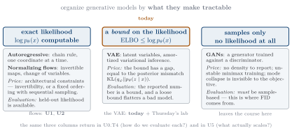
Regime	Families	What you pay	How you must evaluate
Exact likelihood	autoregressive models; normalizing flows (U1, U2)	architectural constraints: invertibility, or a fixed ordering with sequential sampling	held-out log-likelihood is available and meaningful
A bound	VAE (today)	a gap equal to \(\mathrm{KL}(q_\varphi \| p_\theta(z \mid x))\), unmeasurable in general	the reported number is a bound; a loose bound flatters a bad model
Samples only	GANs	no density at all; unstable minimax training	sample-based metrics are the only option — this is where FID comes from

Flow Matching, when we reach it in U3, will not fit neatly into any row — which is a large part of why it won.

GANs

A generator \(G_\psi\) maps noise to samples, \(z \sim p(z) \mapsto G_\psi(z)\), and never defines a density. A discriminator \(D_\omega\) is trained to tell generated samples from real ones. The two play a minimax game (Goodfellow et al. 2014):

\[ \min_{\psi} \max_{\omega} \;\; \mathbb{E}_{x \sim q}\big[\log D_\omega(x)\big] \;+\; \mathbb{E}_{z \sim p(z)}\big[\log\big(1 - D_\omega(G_\psi(z))\big)\big]. \tag{12}\]

Three consequences, which is all we need:

• Likelihood-free. There is no \(p_\psi(x)\) to report, so evaluation must be based on samples. This is the historical origin of FID, which U0.T4 defines properly.
• Training instability. Equation 12 is not the minimization of any single objective, so the usual convergence intuitions from U0.T2 do not transfer. Two networks chasing each other can oscillate indefinitely.
• Mode collapse. A generator that produces only a few of the data’s modes can still fool the discriminator. Nothing in Equation 12 penalizes missing coverage — the failure is invisible to the objective, which is exactly why it needs an external metric to detect.

Autoregressive models

Factor the joint by the chain rule, without approximation, along a fixed ordering of the \(d\) coordinates:

\[ p_\theta(x) \;=\; \prod_{i=1}^{d} p_\theta\big(x_i \mid x_{<i}\big). \tag{13}\]

Each factor is a small conditional distribution produced by a network reading only earlier coordinates. This gives an exact likelihood, which is why autoregressive models remain the reference point for density estimation. The catch is the asymmetry of the two directions:

• Evaluating \(\log p_\theta(x)\) is fast: all \(d\) conditionals can be computed in one parallel pass, since every \(x_{<i}\) is already known.
• Sampling is slow: coordinate \(i\) cannot be drawn until \(x_{<i}\) exists, so generation costs \(d\) sequential passes. For an image, that is one pass per pixel.

There is the planted sentence again, in its other orientation: fast to evaluate, slow to sample.

The autoregressive “one fast direction” tradeoff does not stay in this session — it reappears inside flow architectures in U1.T2, where masked autoregressive flows (fast density, slow sampling) and inverse autoregressive flows (fast sampling, slow density) are the same coin, and the choice between them is made by asking which direction your application needs. GANs, by contrast, leave the course here; they return only as the reason we need sample-based evaluation at all.

The VAE, assembled

Every piece is now on the table.

Components. Prior \(p(z) = \mathcal{N}(0, I_{d_z})\); encoder \(q_\varphi(z \mid x) = \mathcal{N}\big(z; \mu_\varphi(x), \operatorname{diag}(\sigma_\varphi(x)^2)\big)\); decoder \(p_\theta(x \mid z)\).

Training objective (minimized over \(\theta, \varphi\) jointly): \[ \begin{aligned} \mathcal{L}_{\mathrm{VAE}}(\theta, \varphi) \;=\; -\,\mathbb{E}_{x \sim q}\Big[\; &\mathbb{E}_{\varepsilon \sim \mathcal{N}(0, I)}\big[ \log p_\theta\big(x \mid \mu_\varphi(x) + \sigma_\varphi(x) \odot \varepsilon\big)\big] \\[2pt] &\;-\; \mathrm{KL}\big(q_\varphi(z \mid x) \,\big\|\, p(z)\big) \;\Big]. \end{aligned} \]

Gradient path. The inner expectation is reparameterized (Equation 10), so \(\nabla_\varphi\) reaches \(\mu_\varphi, \sigma_\varphi\) through \(z\); the KL term is closed-form (Equation 6) and differentiable directly.

Sampling (no encoder involved): draw \(z \sim \mathcal{N}(0, I_{d_z})\), then \(x \sim p_\theta(x \mid z)\).

Two properties are worth stating plainly. The training objective is the negative ELBO averaged over data, so minimizing it maximizes a lower bound on Equation 1 — we never optimize the thing we actually want, only something provably below it. And the encoder, which the entire derivation was built around, plays no part in generation: it is scaffolding for training, discarded at sampling time.

What the next session builds, and where this goes

U0.L3 implements exactly this object on MNIST, trained with the hygiene-stack from U0.L2 — configuration, seeding, MLflow logging, checkpointing. Two specifics to expect. The loss will return its parts, {loss, recon, kl}, not a single scalar, per the composite-loss rule. And the KL term will be logged per latent dimension, because its behaviour dimension-by-dimension shows something the aggregate hides. That is the next session’s discussion, not today’s.

The assignment assembles itself across the unit: PS0 is the U0.L3 VAE (vae-mnist-scratch), with the U-Net encoder you build in U0.L4 (unet-skeleton), trained with the U0.L2 hygiene stack, and evaluated with the FID harness you also build in U0.L4 (eval-harness). Grading is on correctness and reproducibility — configuration, seed, commit, and logged run — not on how good the samples look.

And the one line to carry forward from today, because two later sessions cite it by name: the bound in Equation 7 has a gap, the gap is exactly a posterior mismatch, and asking what the gap is is a habit this course will keep asking you to exercise.

Further reading

• (Bishop and Bishop 2024), chapters on latent-variable models and deep generative models — the closest match to today’s level and notation.
• (Murphy 2023) — considerably more depth on variational inference, including the material UP.A will cover formally.
• (Kingma and Welling 2014) and (Rezende, Mohamed, and Wierstra 2014) — the two 2014 papers that introduced amortized variational inference with the reparameterized gradient, independently and within months of each other.
• (Goodfellow et al. 2014) — the GAN paper, for Equation 12 and the likelihood-free framing.

References

Bishop, Christopher M., and Hugh Bishop. 2024. Deep Learning: Foundations and Concepts. Springer. https://doi.org/10.1007/978-3-031-45468-4.

Goodfellow, Ian J., Jean Pouget-Abadie, Mehdi Mirza, Bing Xu, David Warde-Farley, Sherjil Ozair, Aaron Courville, and Yoshua Bengio. 2014. “Generative Adversarial Nets.” In Advances in Neural Information Processing Systems. https://arxiv.org/abs/1406.2661.

Kingma, Diederik P., and Max Welling. 2014. “Auto-Encoding Variational Bayes.” In International Conference on Learning Representations. https://arxiv.org/abs/1312.6114.

Murphy, Kevin P. 2023. Probabilistic Machine Learning: Advanced Topics. MIT Press.

Rezende, Danilo Jimenez, Shakir Mohamed, and Daan Wierstra. 2014. “Stochastic Backpropagation and Approximate Inference in Deep Generative Models.” In International Conference on Machine Learning. https://arxiv.org/abs/1401.4082.

Footnotes

1. The manipulation requires \(q_\varphi(z \mid x) > 0\) wherever \(p_\theta(x \mid z)\, p(z) > 0\), so that dividing by \(q_\varphi\) is legitimate. A full-support Gaussian encoder satisfies this automatically, which is one practical reason the Gaussian family is the default.