U0.T3 — Latent Variables and the VAE

Flow-Based Generative Models · UFRJ · 2026.2

01From functions to distributions

Two sessions ago, and today

U0.T1–U0.T2. We fit a function \(f_\theta \colon x \mapsto y\) and judged it by prediction. Optimizers, schedules, initialization, normalization — all of that machinery still applies, unchanged.

Today. We fit a distribution \(p_\theta \approx q\) and judge it by how well it explains. The maximum-likelihood template from U0.T1, written without labels:

\[ \max_{\theta} \; \mathbb{E}_{x \sim q}\big[\log p_\theta(x)\big] . \]

Nothing above is new. What is new: the objective is no longer computable.

Recall U0.T1’s MLE board formula and re-show it if it is still on a board. The point of this slide is that the optimization stack does not change today — only the objective becomes an object we cannot evaluate. Everything in the next 85 minutes is a response to that.

The sentence I planted in U0.T1

“Much of this course is about what to do when the model’s likelihood is easy to sample but hard to evaluate — or vice versa.”

Today it stops being a slogan. The VAE is our first concrete instance of the first half; autoregressive models, at the end of the hour, are the second half.

Question of the day: when \(\log p_\theta(x)\) cannot be computed, what exactly do we optimize instead — and what do we give up by doing so?

Say the answer’s shape now: we optimize a lower bound, and the amount we give up is an identified quantity. That identity is the session’s boxed result, Block C.

02Latent-variable models

The modeling move

Build something complicated by marginalizing a hidden variable:

Prior \(p(z) = \mathcal{N}(0, I_{d_z})\) on a latent space; decoder \(p_\theta(x \mid z)\) on \(\mathbb{R}^d\). The model is the marginal \[ p_\theta(x) = \int p_\theta(x \mid z)\, p(z)\, \mathrm{d}z = \mathbb{E}_{z \sim p(z)}\big[p_\theta(x \mid z)\big]. \] Sampling is trivial: draw \(z \sim p(z)\), then \(x \sim p_\theta(x \mid z)\).

Each piece is as simple as a distribution gets — a standard Gaussian, and \(\mathcal{N}(g_\theta(z), \sigma^2 I)\) for a network \(g_\theta\).

Stress “sampling is trivial” and let it sit — it is half of the planted sentence, delivered on the second slide of the block. Board 1 starts here: write the marginalization integral and leave it up through Block C.

The expressivity is in the marginalization

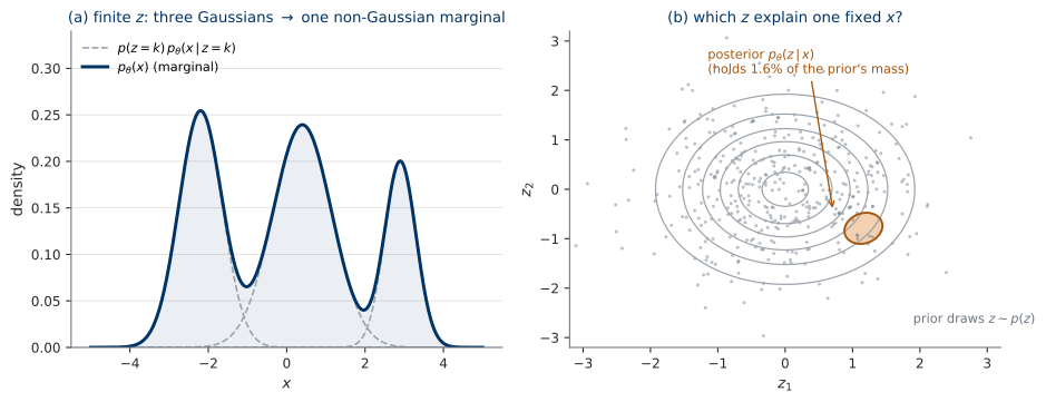
Three Gaussians in, one multimodal distribution out — the parts are simple, the marginal is not.

(b) is the whole problem: the \(z\) explaining one fixed \(x\) (orange) hold 1.6% of the prior’s mass.

The obvious estimator

The marginal is an expectation, so estimate it. Draw \(z_1, \dots, z_K \sim p(z)\):

\[ \widehat{p}_\theta(x) = \frac{1}{K} \sum_{k=1}^{K} p_\theta(x \mid z_k), \qquad \mathbb{E}_{z_{1:K} \sim p(z)}\big[\widehat{p}_\theta(x)\big] = p_\theta(x). \]

Unbiased. Also useless:

• \(p_\theta(x \mid z)\) is sharply peaked in \(z\) — almost every term is numerically zero.
• Whether the estimate is any good depends on whether any draw landed in the orange region.
• And we need \(\log \widehat{p}_\theta(x)\), which is not even unbiased for \(\log p_\theta(x)\).

The last bullet matters and gets skipped in most treatments: Jensen bites in the wrong direction here — the log of an unbiased estimator is biased downward, by an amount growing with the variance we just failed to control. So “unbiased but noisy” is not a partial solution.

Not a rhetorical claim — a measured one

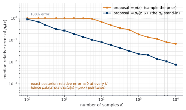
A linear decoder \(g_\theta(z) = Az + b\), chosen so \(p_\theta(x)\) is known exactly. At \(K = 100\): prior sampling is \(68\%\) wrong, posterior-guided sampling \(8\%\).

Two things to say out loud. (1) The flat stretch at 100% error is the regime where no draw has landed in the explaining region at all — the estimate is essentially zero. (2) The toy is linear ONLY so a ground truth exists; swap in a network and the reference line, the exact posterior, and the closed-form marginal all vanish at once. That vanishing is the session.

What would fix it

Sample from a proposal \(r\) instead of the prior, and reweight:

\[ p_\theta(x) = \mathbb{E}_{z \sim r}\!\left[\frac{p_\theta(x \mid z)\, p(z)}{r(z)}\right]. \]

Take \(r = p_\theta(\cdot \mid x)\), the true posterior. By Bayes’ rule the ratio equals \(p_\theta(x)\) for every \(z\):

\[ \frac{p_\theta(x \mid z)\, p(z)}{p_\theta(z \mid x)} = p_\theta(x) \quad \Longrightarrow \quad \text{zero variance. One sample suffices.} \]

So the posterior is exactly the object we want.

Pause here. This is the strongest possible motivation for the posterior, and it is rarely stated this sharply: the posterior is not “a helpful auxiliary distribution”, it is the unique proposal that makes the problem free. Next slide destroys it.

And exactly the object we cannot have

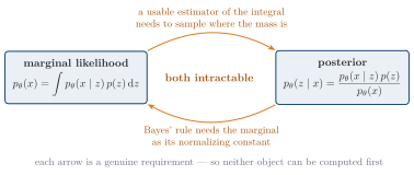
Bayes’ rule computes the posterior from the marginal — which is what we were trying to find.

Board 1’s diagram. Keep it visible through Block C: the ELBO is the answer to THIS board. If someone asks “why not iterate?” — that is a real question, and the honest answer is that the fixed point is not accessible either; the VAE’s move is to stop trying.

Why this matters later

U1’s answer is invertibility. Build \(p_\theta\) from a bijection; the change-of-variables formula returns \(\log p_\theta(x)\) exactly, with no marginalization at all.

The VAE’s answer is bounding. Give up computing \(\log p_\theta(x)\); optimize a tractable lower bound instead.

Keep both on your map. Much of this course is a tour of such answers — and Flow Matching’s, in U3, is a third one that sidesteps the likelihood entirely.

03The ELBO

First: a notation collision, resolved

The course reserves unsubscripted \(q\) for the data distribution. The VAE literature uses \(q\) for the encoder. Both appear in every equation for the next 25 minutes.

• \(q\) unsubscripted \(=\) the data distribution, samples \(x \sim q\).
• Encoder and variational distributions always carry their subscript: \(q_\varphi(z \mid x)\).
• Decoder \(p_\theta(x \mid z)\); prior \(p(z) = \mathcal{N}(0, I_{d_z})\).

Thirty seconds well spent: this is why we can put diffusion and flow matching in the same equations in U3 without a symbol quietly changing meaning.

Derivation 1 — insert \(q_\varphi\), apply Jensen

\[ \begin{aligned} \log p_\theta(x) &= \log \int q_\varphi(z \mid x)\, \frac{p_\theta(x \mid z)\, p(z)}{q_\varphi(z \mid x)}\, \mathrm{d}z = \log\, \mathbb{E}_{z \sim q_\varphi(\cdot \mid x)}\!\left[ \frac{p_\theta(x \mid z)\, p(z)}{q_\varphi(z \mid x)}\right] \\[4pt] &\ \ge\ \mathbb{E}_{z \sim q_\varphi(\cdot \mid x)}\!\left[ \log \frac{p_\theta(x \mid z)\, p(z)}{q_\varphi(z \mid x)}\right] &&\text{(Jensen; } \log \text{ concave)} \\[4pt] &= \underbrace{\mathbb{E}_{z \sim q_\varphi(\cdot \mid x)}\big[\log p_\theta(x \mid z)\big] - \mathrm{KL}\big(q_\varphi(z \mid x) \,\big\|\, p(z)\big)}_{\textstyle \mathrm{ELBO}(\theta, \varphi; x)} \end{aligned} \]

\(q_\varphi\) is arbitrary so far. Both terms are computable: we can sample \(q_\varphi\) because we designed it, and the KL of two Gaussians is closed-form.

“Evidence lower bound” — evidence is the classical name for the marginal likelihood. Note the support condition out loud: we need q_φ > 0 wherever the numerator is, which a full-support Gaussian gives for free — one practical reason the Gaussian family is the default.

The one KL fact we need, in three lines

\(\mathrm{KL}(a \,\|\, b) \ge 0\), with equality iff \(a = b\) almost everywhere.

\[ -\mathrm{KL}(a \,\|\, b) = \mathbb{E}_{y \sim a}\!\left[\log \frac{b(y)}{a(y)}\right] \;\le\; \log\, \mathbb{E}_{y \sim a}\!\left[\frac{b(y)}{a(y)}\right] = \log \int b = 0 . \]

KL gets its full treatment in UP.A — including the Gaussian closed forms you will use in the next lab (U0.L3) as black boxes, and the sense in which it is not a distance.

Strict concavity gives the equality case. Do not spend more than 90 seconds here — it is bookkeeping, not levelling. The UP.A flag is the point: PGMAT students get the tool now and the theory in the joint phase.

Derivation 2 — how big is the gap?

Jensen says the bound exists. It does not say what we lost. Start from the KL to the true posterior and substitute Bayes’ rule:

\[ \begin{aligned} \mathrm{KL}\big(q_\varphi(z \mid x) \,\big\|\, p_\theta(z \mid x)\big) &= \mathbb{E}_{z \sim q_\varphi(\cdot \mid x)}\big[\log q_\varphi(z \mid x) - \log p_\theta(z \mid x)\big] \\[2pt] &= \mathbb{E}_{z \sim q_\varphi(\cdot \mid x)}\big[\log q_\varphi(z \mid x) - \log p_\theta(x \mid z) - \log p(z) + \log p_\theta(x)\big] \\[2pt] &= -\,\mathbb{E}_{z \sim q_\varphi(\cdot \mid x)}\!\left[ \log \frac{p_\theta(x \mid z)\, p(z)}{q_\varphi(z \mid x)}\right] + \log p_\theta(x) \\[2pt] &= -\,\mathrm{ELBO}(\theta, \varphi; x) + \log p_\theta(x) . \end{aligned} \]

Line 3 uses that \(\log p_\theta(x)\) is constant in \(z\); line 4 is the definition. Rearrange.

BOARD 2 — do this live, all four lines, and do not erase it. Point back at it during the Block F assembly slide. It is four lines from the definitions, and every student should be able to reproduce it cold; that is the assessment-relevant skill from today.

The gap identity

For every \(\theta\), every \(\varphi\), and every \(x\) with \(p_\theta(x) > 0\): \[ \log p_\theta(x) = \mathrm{ELBO}(\theta, \varphi; x) + \mathrm{KL}\big(q_\varphi(z \mid x) \,\big\|\, p_\theta(z \mid x)\big). \] The slack is exactly the divergence from \(q_\varphi\) to the true posterior.

Since \(\mathrm{KL} \ge 0\), this re-proves \(\mathrm{ELBO} \le \log p_\theta(x)\) for free. The two derivations are not redundant: the first shows the bound exists, the second identifies it.

This box is the session’s produced artifact, elbo-derivation. It is cited by name in U3.T2 and U5.T1 — tell them it will come back, without saying how.

Read it twice, in both directions

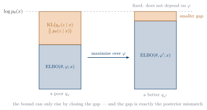
Over \(\varphi\): the left side does not depend on \(\varphi\) — maximizing the ELBO can only shrink the gap. Optimizing the encoder is approximate posterior inference.

At fixed \(\varphi\): the number we report falls short by exactly the posterior mismatch.

Then state the habit, and mean it: whenever this course hands you a bound, ask what the gap IS. A bound with an identified gap is a scientific object; a bound with an unknown gap is a number that flatters you. This recurs — U1’s bpd, U3’s detour losses.

The same thing, moving

Real gradient ascent on the ELBO over a diagonal qφ, on the same linear-decoder toy as the static figures — every number is computed, not drawn. Two things to point at. (1) The dashed ceiling never moves: that is the identity’s content, and it kills the common misreading that optimizing φ raises the likelihood. (2) The ending is honest: the mean converges exactly, the shape cannot, and 0.013 nats survive — the floor for ANY diagonal family here. Small number, but the qualitative failure is visible in the tilt.

Anatomy: two terms pulling opposite ways

\[ \mathrm{ELBO}(\theta, \varphi; x) = \underbrace{\mathbb{E}_{z \sim q_\varphi(\cdot \mid x)}\big[\log p_\theta(x \mid z)\big]}_{\text{reconstruction}} \;-\; \underbrace{\mathrm{KL}\big(q_\varphi(z \mid x) \,\big\|\, p(z)\big)}_{\text{stay near the prior}} \]

• Reconstruction alone wants an encoder that packs everything about \(x\) into \(z\).
• KL alone wants an encoder that ignores \(x\) and returns the prior — at which point the latent carries no information.

Where training settles is a property of the model and the data, not something we set.

Course rule (U0.T2 recipe card): composite losses log their parts. Never log only the sum.

Amortization: from an identity to an algorithm

Classical variational inference optimizes a separate \(q^{(i)}(z)\) per datapoint — an inner loop at training and test time, useless on unseen \(x\).

The VAE’s move (Kingma and Welling 2014; Rezende, Mohamed, and Wierstra 2014): replace that optimization with a network.

\[ x \;\longmapsto\; \big(\mu_\varphi(x),\, \sigma_\varphi(x)\big), \qquad q_\varphi(z \mid x) = \mathcal{N}\big(z;\, \mu_\varphi(x),\, \operatorname{diag}(\sigma_\varphi(x)^2)\big). \]

One forward pass, any \(x\), including one never seen. The cost of inference is amortized across the dataset.

Flag the pattern as transferable: “replace a per-instance optimization by a network trained to predict its solution” is one of the field’s most reused moves — they will meet it again. Mention the amortization gap by name only, so the term does not surprise them in a paper.

One flag, planted and left

A variational bound plus Gaussian algebra returns in the D2 detour of U3, where the surprising punchline will be about the weighting of the resulting loss — not its minimizer.

That is the entire flag. Nothing more is claimed, and guessing the rest will not help you.

Gray-teaser protocol, same visual language as U0.T1’s foreshadowing slide and U0.T2’s residual-connection teaser. Say the sentence, do not elaborate, move on. If pushed: smile, “U3.T2”. Forbidden today: any claim that diffusion IS a hierarchical VAE; any mention of score, noising, or denoising.

04Reparameterization

The gradient we cannot take

Training needs \(\nabla_\varphi \mathrm{ELBO}\), and the reconstruction term has the shape

\[ \nabla_\varphi \, \mathbb{E}_{z \sim q_\varphi(\cdot \mid x)}\big[f(z)\big], \qquad f(z) = \log p_\theta(x \mid z). \]

Compare with every gradient U0.T1 taught you:

• There: \(\varphi\) was in the integrand; \(\nabla\) and \(\mathbb{E}\) commuted.
• Here: \(\varphi\) indexes the distribution being sampled from, and does not appear in \(f\) at all.

Write \(\frac{1}{K}\sum_k f(z_k)\), call .backward(), get zero — correctly, since \(f\) really does not depend on \(\varphi\).

This is the single most common conceptual gap in a first VAE implementation, and the “correctly zero” framing is what fixes it: autograd is not failing, the graph genuinely has no path. Board 3 starts here.

The device: change the sampling variable

Let \(\varepsilon \sim \mathcal{N}(0, I_{d_z})\) — a law carrying no parameters — and set \[ z = \mu_\varphi(x) + \sigma_\varphi(x) \odot \varepsilon \quad \Longrightarrow \quad z \sim q_\varphi(z \mid x). \] Then, for integrable \(f\), \[ \nabla_\varphi \, \mathbb{E}_{z \sim q_\varphi(\cdot \mid x)}\big[f(z)\big] = \mathbb{E}_{\varepsilon \sim \mathcal{N}(0, I)}\big[ \nabla_\varphi\, f\big(\mu_\varphi(x) + \sigma_\varphi(x) \odot \varepsilon\big)\big]. \]

The exchange is now the ordinary one: the measure is \(\mathcal{N}(0, I)\), fixed and \(\varphi\)-free. Everything \(\varphi\)-dependent moved inside \(f\), where autodiff can reach it.

In the computational graph

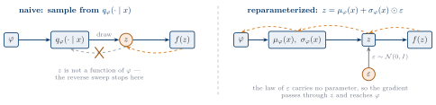
The graph now contains a random input. We changed no distribution — only which quantities the graph treats as given.

Board 3’s sketch. Explicitly connect to U0.T1: this is the same forward-blue/backward-orange cotangent picture from the autodiff session, with exactly one node changed. The general framing is what to remember — “reparameterize the sampling variable, then push the gradient inside” — and it works for any law expressible as a differentiable transform of a parameter-free base.

Watch the sweep stop, then not stop

Deliberately the same visual grammar as U0.T1’s ReverseModeSweep — say so out loud, because the point is that this is the same sweep meeting a new obstacle. The beat that matters is the pulse dying at z and ∇φ = 0 appearing: autograd is not failing there, the graph genuinely has no path. Then ε enters as an input, z becomes an ordinary node, and the same pulse reaches φ.

The general alternative, named only

When no such transform exists — discrete latents, most obviously — the fallback is the score-function (REINFORCE) estimator:

\[ \nabla_\varphi \, \mathbb{E}_{z \sim q_\varphi(\cdot \mid x)}\big[f(z)\big] = \mathbb{E}_{z \sim q_\varphi(\cdot \mid x)}\big[f(z)\, \nabla_\varphi \log q_\varphi(z \mid x)\big]. \]

Fully general, needs no differentiable path through \(z\) — and badly high-variance without careful control variates. That is why we reparameterize wherever we can.

Why this matters later

Every loss in the main course is an expectation over sampled quantities — in Flow Matching, \(\mathbb{E}_{t,\, x_0,\, x_1}\) over a time, a noise sample, and a data sample. Reparameterized sampling is how such objectives become trainable code rather than integrals on a page.

By U3 this will be so routine that the interesting question is no longer how to differentiate through a sample, but which sampling distribution to choose.

05Panorama: the landscape

Organize by what a model makes tractable

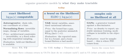
Not by architecture. Not by chronology. By what you can compute.

This taxonomy slide is the block’s real deliverable — it returns in U0.T4 (each column dictates how you can evaluate) and in U5 (each column’s scaling behaviour). Hard cap on this block: 20 minutes, two slides per family, no variants, no training tips. If it runs long, cut GAN detail, not the taxonomy.

GANs: the generator/discriminator game

A generator \(G_\psi\) maps noise to samples and never defines a density; a discriminator \(D_\omega\) learns to tell fake from real (Goodfellow et al. 2014):

\[ \min_{\psi} \max_{\omega} \;\; \mathbb{E}_{x \sim q}\big[\log D_\omega(x)\big] + \mathbb{E}_{z \sim p(z)}\big[\log\big(1 - D_\omega(G_\psi(z))\big)\big]. \]

Note the expectations still carry their subscripts — the discipline does not lapse for a slide about someone else’s model.

GANs: three consequences

• Likelihood-free. No \(p_\psi(x)\) to report, so evaluation must be sample-based. This is where FID comes from — U0.T4 defines it properly.
• Training instability. A minimax problem is not the minimization of any single objective; U0.T2’s convergence intuitions do not transfer. Two networks can chase each other indefinitely.
• Mode collapse. A generator covering only a few modes still fools the discriminator. Nothing in the objective penalizes missing coverage — the failure is invisible to the loss, which is precisely why an external metric is needed.

The third bullet is the one that plants U0.T4: a model whose objective cannot see its own worst failure mode is the argument for FID existing at all. Do not go into WGAN, spectral norm, or any variant.

Autoregressive models: exact, by the chain rule

Factor the joint along a fixed ordering of the \(d\) coordinates — no approximation anywhere:

\[ p_\theta(x) = \prod_{i=1}^{d} p_\theta\big(x_i \mid x_{<i}\big). \]

Each factor is a small conditional produced by a network reading only earlier coordinates. The likelihood is exact, which is why these remain the reference point for density estimation.

Autoregressive models: the asymmetry

• Evaluating \(\log p_\theta(x)\) is fast — all \(d\) conditionals compute in one parallel pass, since every \(x_{<i}\) is already known.
• Sampling is slow — coordinate \(i\) waits for \(x_{<i}\), so generation costs \(d\) sequential passes. For an image: one pass per pixel.

There is the planted sentence in its other orientation: fast to evaluate, slow to sample.

This one-fast-direction tradeoff reappears inside flow architectures in U1.T2 — masked autoregressive flows (fast density, slow sampling) against inverse autoregressive flows (fast sampling, slow density). GANs leave the course here, surviving only as the reason sample-based evaluation exists.

06The VAE, assembled

Every piece, on one slide

Components. \(p(z) = \mathcal{N}(0, I_{d_z})\); encoder \(q_\varphi(z \mid x) = \mathcal{N}\big(z; \mu_\varphi(x), \operatorname{diag}(\sigma_\varphi(x)^2)\big)\); decoder \(p_\theta(x \mid z)\).

Objective (minimized over \(\theta, \varphi\) jointly): \[ \mathcal{L}_{\mathrm{VAE}}(\theta, \varphi) = -\,\mathbb{E}_{x \sim q}\Big[ \mathbb{E}_{\varepsilon \sim \mathcal{N}(0, I)}\big[ \log p_\theta\big(x \mid \mu_\varphi(x) + \sigma_\varphi(x) \odot \varepsilon\big)\big] - \mathrm{KL}\big(q_\varphi(z \mid x) \,\big\|\, p(z)\big) \Big] \]

Sampling (no encoder): \(z \sim \mathcal{N}(0, I_{d_z})\), then \(x \sim p_\theta(x \mid z)\).

We never optimize what we want — only something provably below it. And the encoder, which the whole derivation was built around, plays no part in generation.

Point back at Board 2 (the gap identity) while saying the first sentence. The second sentence surprises people every year: the encoder is training scaffolding, discarded at sampling time.

Next session: this exact object, on MNIST

U0.L3 implements it, trained with the hygiene-stack from U0.L2 — config, seeding, MLflow logging, checkpointing.

Two specifics to expect:

• The loss returns its parts, {loss, recon, kl} — not a single scalar.
• The KL term is logged per latent dimension, because its dimension-by-dimension behaviour shows something the aggregate hides.

That last one is the next session’s discussion (U0.L3), not today’s.

PS0 is assembling itself

From	Artifact	Role in PS0
U0.L2	hygiene-stack	“trained with the hygiene stack”
U0.L3	vae-mnist-scratch	the model — next session
U0.L4	unet-skeleton	your own encoder, swapped in
U0.L4	eval-harness	FID at the course-standard sample count

Graded on correctness and reproducibility — config, seed, commit, logged run — not on how good the samples look.

What to carry out of this room

1. The latent-variable frame: expressivity from marginalization, at the cost of an intractable integral.
2. The gap identity — reproduce its four lines cold: \(\log p_\theta(x) = \mathrm{ELBO} + \mathrm{KL}(q_\varphi \| p_\theta(z \mid x))\).
3. Reparameterization as a general device: change the sampling variable, then push the gradient inside.
4. The habit: whenever you are handed a bound, ask what the gap is.

Exit line. Item 4 is the one that recurs furthest — it is the question that makes the D2 punchline land in U3.T2, and it is the reason the identity was proved rather than merely stated.

References

Goodfellow, Ian J., Jean Pouget-Abadie, Mehdi Mirza, Bing Xu, David Warde-Farley, Sherjil Ozair, Aaron Courville, and Yoshua Bengio. 2014. “Generative Adversarial Nets.” In Advances in Neural Information Processing Systems. https://arxiv.org/abs/1406.2661.

Kingma, Diederik P., and Max Welling. 2014. “Auto-Encoding Variational Bayes.” In International Conference on Learning Representations. https://arxiv.org/abs/1312.6114.

Rezende, Danilo Jimenez, Shakir Mohamed, and Daan Wierstra. 2014. “Stochastic Backpropagation and Approximate Inference in Deep Generative Models.” In International Conference on Machine Learning. https://arxiv.org/abs/1401.4082.