U0.T4 — Architectures for the Road and Evaluation
Session U0.T4 · date: see calendar-map
This is the parts-list session. Everything the course trains after the bootcamp is assembled from the components below, and everything it generates is judged by the metrics below. Two of those components will be handed to you as code contracts rather than as prose, so this page is written to be the reference you return to when the code stops making sense.
The session has two deliverables that later sessions cite by name. The first is time-conditioning-patterns (Section 4): the sinusoidal ladder, the FiLM/AdaGN modulation, and the rule for adding a second conditioning signal. It is the single most transferable box of the bootcamp, because every velocity field and every score network you will read is built this way. The second is fid-definition (Section 6.2): the Fréchet Inception Distance with its caveats, which becomes the documentation of the evaluation harness you build in the next lab session (U0.L4).
Standing references for the unit: (Bishop and Bishop 2024; Murphy 2023). The primary sources for today’s objects are (Vaswani et al. 2017) for attention, (Ronneberger, Fischer, and Brox 2015) for the U-Net, (Perez et al. 2018) for feature-wise modulation, (Peebles and Xie 2023) for the transformer backbone and its conditioning, (Heusel et al. 2017) for FID, (Theis, Oord, and Bethge 2016) for the limits of likelihood, and (Kynkäänniemi et al. 2019) for manifold precision and recall.
One signature, for the rest of the course
Write this down and keep it. Every network the course trains from here on has the same shape:
\[ f_\theta \colon \; \underbrace{(B, C, H, W)}_{x} \; \times \; \underbrace{(B,)}_{t} \; \longrightarrow \; (B, C, H, W) . \tag{1}\]
An input of some shape, a time argument, and an output of the same shape as the input. When the course reaches Flow Matching, the object with this signature is the learned velocity field \(u_t^\theta(x)\); in the diffusion detours it is a score or noise network; today it is just “the network”. The two questions this session answers are: what goes inside, and how does \(t\) get in.
In every network signature in this course, t is a (B,) tensor of floats in \([0,1]\), with \(t=0\) at noise and \(t=1\) at data. Not an integer index, not a step count, not a shape-\((B,1,1,1)\) broadcast — a flat vector of floats. Code that needs any other time variable converts outside the network.
The reason for the strictness is not tidiness. The diffusion literature counts time backwards in discrete steps, and the moment a network accepts an integer timestep, that convention has entered the codebase and every later translation becomes a source of silent sign errors. The next lab session (U0.L4) enforces this line with an assertion inside unet-skeleton.
The second question of the session is separate and equally practical: given a trained generative model, how do we know it is any good? Section 6 gives three answers and is honest about what each one misses.
Attention, in one pass
Attention appears in this course as vocabulary. It sits at the low-resolution stages of the U-Net, it is the whole of the transformer backbone in Section 5, and it is assumed without comment by most of the seminar literature in U6. This section is the only place the course derives it; after this it is a word.
The operation
Start from a concrete need. A convolution mixes a pixel with its neighbours, and its reach grows only by stacking layers. Sometimes a position needs information from a distant position, chosen by content rather than by geometry — and which position that is depends on the data, not on the architecture. Attention is the mechanism that lets a position ask for what it needs.
Each of the \(n\) positions produces three vectors by linear maps of its own representation: a query \(q_i \in \mathbb{R}^{d_k}\), saying what this position is looking for; a key \(k_j \in \mathbb{R}^{d_k}\), advertising what position \(j\) has; and a value \(v_j \in \mathbb{R}^{d_v}\), the content that position \(j\) will hand over. Stack them as rows of \(Q, K, V\).
\[ \operatorname{Attn}(Q, K, V) \;=\; \operatorname{softmax}\!\left( \frac{Q K^{\top}}{\sqrt{d_k}} \right) V . \tag{2}\] The matrix \(A = \operatorname{softmax}(QK^\top/\sqrt{d_k})\) has non-negative rows that sum to one, so the output at position \(i\) is a convex combination of the value vectors, with weights chosen by how well \(q_i\) matches each \(k_j\).
Two details earn their place. The softmax turns raw match scores into a probability distribution over positions, so the output is an average rather than an unbounded sum. The division by \(\sqrt{d_k}\) keeps that softmax usable: if the entries of \(q\) and \(k\) are roughly independent with unit variance, the dot product \(q \cdot k\) has variance \(d_k\), so without the scaling the scores grow with the width, the softmax saturates, and the gradient through it vanishes. The scaling is a variance-propagation argument of exactly the kind U0.T2 made for initialization.
A worked example, small enough to check by hand
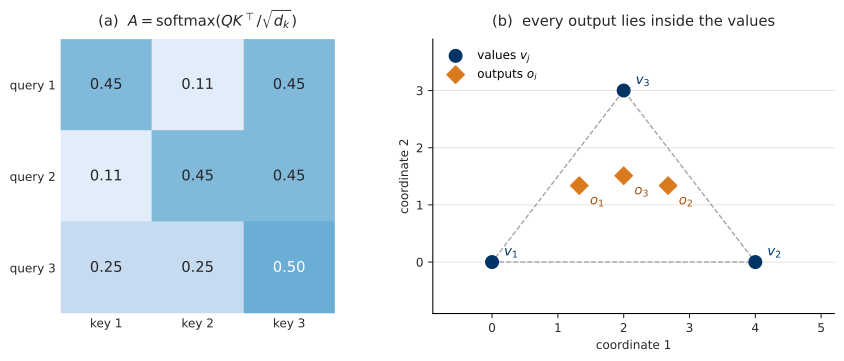
Take three positions and \(d_k = d_v = 2\), with
\[ Q = \begin{pmatrix} 2 & 0 \\ 0 & 2 \\ 1 & 1 \end{pmatrix}, \quad K = \begin{pmatrix} 1 & 0 \\ 0 & 1 \\ 1 & 1 \end{pmatrix}, \quad V = \begin{pmatrix} 0 & 0 \\ 4 & 0 \\ 2 & 3 \end{pmatrix} . \]
Figure 1 shows the result. Query 1 matches key 1 and key 3 equally and largely ignores key 2; query 3, which points between the two axes, splits its attention and puts half of it on key 3. The right panel is the part worth remembering: because each row of \(A\) is a probability vector, every output lies inside the triangle spanned by the value vectors. Attention cannot invent content. It can only redistribute what the values already contain.
Multi-head, and what it buys
One attention operation produces one set of weights, so it can express one notion of relevance at a time. Multi-head attention runs \(h\) copies in parallel on projections of the input into \(h\) lower-dimensional subspaces, then concatenates the results and applies a final linear map:
\[ \begin{aligned} \operatorname{head}_m &= \operatorname{Attn}(X W^Q_m,\; X W^K_m,\; X W^V_m), \\ \operatorname{MHA}(X) &= \big[\operatorname{head}_1, \dots, \operatorname{head}_h\big] \, W^O . \end{aligned} \tag{3}\]
Each head is free to specialize — one on nearby positions, another on a particular kind of content — and the cost is unchanged, because the per-head width is the full width divided by \(h\).
Permutation equivariance, and why it forces the next section
Equation 2 contains no notion of where a position is. Permute the rows of \(Q\), \(K\) and \(V\) by the same permutation \(\pi\), and the output rows are permuted by \(\pi\) and are otherwise identical. The figure script for Figure 1 checks this numerically, and the discrepancy is exactly zero.
For any permutation matrix \(P\), \(\; \operatorname{Attn}(PQ, PK, PV) = P \operatorname{Attn}(Q, K, V)\).
Consequence: attention has no access to position, or to time, or to any other structure that is not present in its inputs. Anything the network must know has to be injected into the representation. That is the whole subject of Section 4.
The cost, and why resolution decides everything
The matrix \(QK^\top\) has \(n^2\) entries, so attention costs \(O(n^2 d_k)\) time and \(O(n^2)\) memory in the number of positions. For an image treated as a sequence of pixels, \(n = HW\), and the quadratic term becomes decisive very quickly: a \(32 \times 32\) image gives \(n = 1024\) and a million-entry attention matrix per head, while a \(256 \times 256\) image gives \(n = 65\,536\) and four billion entries.
This single fact explains the architecture of Section 3. Attention is affordable exactly where the resolution is low, so a convolutional generator puts attention at the bottom of its resolution ladder and nowhere else. The alternative — pay the cost everywhere, but first reduce \(n\) by grouping pixels into patches — is the transformer route of Section 5.
Where you will meet this again. The seminar papers of U6 are transformer-native and will assume everything above without a word. The architecture of Section 5 is this block repeated.
The U-Net
The shape problem
Equation 1 asks for a map from \((B,C,H,W)\) to \((B,C,H,W)\). That is a demanding request. The output must carry detail — it is a per-pixel quantity, and a blurred version of it is a wrong version of it — while the decision at each pixel depends on global context, because whether a stroke belongs to a 3 or an 8 is not decidable from a \(3 \times 3\) neighbourhood.
A plain stack of convolutions at full resolution has the detail and, as U0.T2’s receptive-field computation showed, needs impractical depth to acquire the context. A downsampling encoder acquires the context quickly and destroys the detail. The U-Net’s answer is to do both and then to reconnect them.
The anatomy
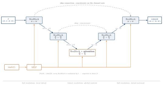
Read Figure 2 left to right. The encoder path alternates ResBlocks with downsampling, halving the spatial resolution and (conventionally) growing the channel count as it goes. The bottleneck sits at the lowest resolution, where every unit sees essentially the whole image and where — by the cost argument of Section 2 — attention is finally affordable. The decoder path mirrors the encoder, upsampling back to full resolution.
The load-bearing part is the dashed arcs. At each resolution, the encoder’s activation is carried directly across to the matching decoder stage and concatenated on the channel axis before the decoder’s ResBlock runs. Concatenation, not addition: the decoder receives the encoder’s features as extra channels and learns what to do with them, rather than having them summed into its own representation on the assumption that the two are commensurate.
Why skips are not optional
The honest argument is about information, and it is short. The bottleneck representation is small by construction. Whatever detail is needed to reconstruct a pixel exactly, and is not predictable from context, cannot survive a passage through it — not because the network is badly trained, but because the representation has fewer numbers in it than the detail requires. The skip connections route that detail around the bottleneck instead of through it.
This makes the U-Net the meeting point of two ideas U0.T2 introduced separately. It is a multiscale architecture, processing the image at several resolutions at once, and it is a residual one, in that each decoder stage receives its input and is asked only for what to change about it.
The interior of a ResBlock
The blocks are not new. Their interior is the U0.T2 recipe card applied without modification:
- GroupNorm, not BatchNorm. The recipe card’s reasoning applies with full force here: a generative model is evaluated one sample at a time, and a normalization whose statistics depend on the rest of the batch makes the output of the network depend on what else was in the batch.
- SiLU as the activation.
- Zero-initialization of the last convolution in each residual branch, so the block begins life as the identity and the untrained network is the zero function.
The one thing Figure 2 adds is the orange path along the bottom. That is Section 4.
Where you will meet this again. This architecture, with the time conditioning of the next section, is unet-skeleton. You build it in the next lab session and train it for the rest of the course.
Time conditioning
This is the section to read twice.
The requirement
The course does not train one network per time. It trains one network for all \(t \in [0,1]\), so \(t\) is an input — a single continuous scalar per example, which has to influence the computation at every layer and every resolution. Two things have to be decided: how to turn one number into something a network can use, and how to deliver it everywhere.
The sinusoidal ladder
Feeding the raw scalar is a bad idea, for a reason worth stating precisely. A single input coordinate enters the first layer through a single column of weights; to make its effect depend on \(t\) in a detailed way, every downstream layer must reconstruct that dependence from one nearly-linear signal. The network can do it, and it wastes capacity doing it.
The standard remedy is to expand \(t\) over a geometric ladder of frequencies, so that both coarse and fine differences in \(t\) are directly available as separate coordinates. It is the same construction transformers use for position, applied to a different variable.
For \(t\) a (B,) tensor of floats in \([0,1]\) and an even width \(d_{\text{emb}}\), with \(\mathrm{half} = d_{\text{emb}}/2\): \[
\begin{aligned}
\omega_k &= (10^4)^{-k/\mathrm{half}}, \qquad k = 0, \dots, \mathrm{half}-1, \\
\mathrm{emb}(t) &= \big[\, \sin(\omega_k \cdot 1000\,t) \,;\; \cos(\omega_k \cdot 1000\,t) \,\big]_{k} .
\end{aligned}
\tag{4}\]
The factor \(1000\) is the only rescale, and it is deliberate. Reference implementations were written for a discrete schedule with about a thousand steps, so their ladder is calibrated to arguments of that magnitude. Multiplying \(t\) by \(1000\) inside the embedding — and nowhere else — makes this from-scratch construction produce the same numbers as those implementations, so that when a later lab cross-checks against a library, a mismatch means a real bug rather than a convention difference. Outside Equation 4, \(t\) is a float in \([0,1]\) everywhere, and the FM arrow is untouched.
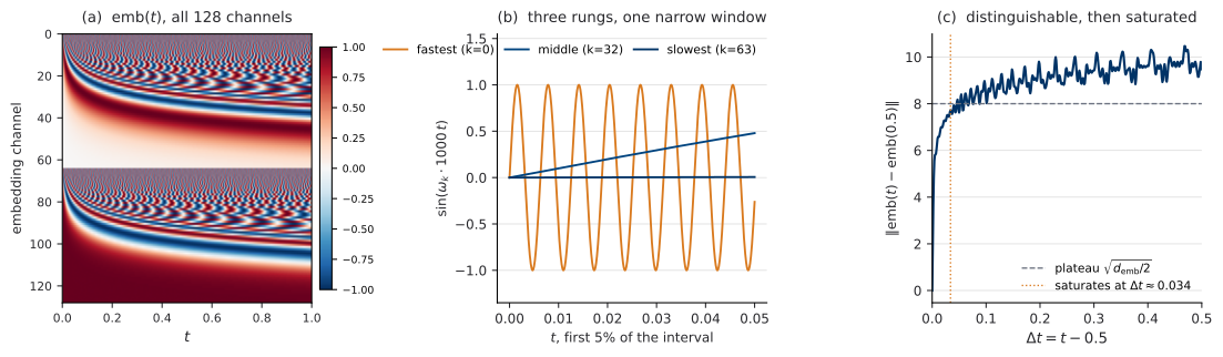
Figure 3 is measured, and it repays a careful look. The slowest rung (\(k = \mathrm{half}-1\)) is monotone across the whole interval and varies by about \(0.12\) radians in total: it is, for practical purposes, a linear encoding of \(t\), and it is what lets the network answer “early or late?”. The fastest rung (\(k=0\)) completes roughly \(159\) cycles over the same interval and resolves differences in \(t\) of order \(10^{-3}\). Everything between interpolates.
The right panel states the honest limit. The distance \(\|\mathrm{emb}(t) - \mathrm{emb}(t')\|\) grows with \(|t - t'|\) only over a short range: it reaches its plateau of \(\sqrt{d_{\text{emb}}/2}\) at about \(\Delta t \approx 0.034\) and stays there. The embedding is not a global ruler for time. It separates nearby times sharply and treats far-apart times as simply different, which is what a conditioning signal needs to do, and it is worth knowing which of the two properties you actually have.
Getting it into every block: FiLM and AdaGN
The embedding now has to reach the computation. Concatenating it to the activations is possible and wasteful: it adds channels at every resolution, and the network has to learn to read them at each one. The mechanism the field settled on is modulation (Perez et al. 2018).
Pass the embedding through a small multilayer perceptron and produce, for each block and each channel, a scale and a shift. Apply them to the normalized activation:
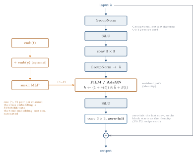
Let \(\hat h\) be the output of the block’s normalization layer. Then \[ h \;\leftarrow\; \big(1 + \gamma(t)\big) \odot \hat h \;+\; \beta(t), \tag{5}\] where \(\gamma(t), \beta(t) \in \mathbb{R}^{C}\) are produced from \(\mathrm{emb}(t)\) by a small learned map, one pair per channel, and \(\odot\) is elementwise over channels.
AdaGN is the name for Equation 5 when the normalization is GroupNorm — that is, FiLM applied at the norm. It is the same operation.
Three observations. The modulation is written as \(1 + \gamma\) rather than \(\gamma\) so that \(\gamma = 0\) means no modulation; combined with zero-initialization of the projection, the block starts out ignoring \(t\) and learns to use it. It is cheap: two numbers per channel per block, against the many thousands in a convolution kernel. And it lands after the normalization, which is the point — normalization has just removed the activation’s scale and offset, and modulation is what puts a \(t\)-dependent scale and offset back.
One more conditioning signal, for free
Suppose the model should also depend on a class label \(y\). Embed \(y\) in a table of the same width, and add it to the time embedding:
\[ c = \mathrm{emb}(t) + \mathrm{emb}(y) , \tag{6}\]
then feed \(c\) through the same projection to the same \((\gamma, \beta)\). Nothing else in the architecture changes. Summing rather than concatenating keeps the width fixed, so the modulation path does not grow with the number of conditioning signals, and it is the convention the reference implementations use.
A class-conditional model built exactly this way returns in U3, where the question becomes what to do with the conditioning at sampling time. That is a later topic and this is all that is needed now.
The artifact
- Ladder. \(\mathrm{emb}(t)\) as in Equation 4: geometric frequencies \(\omega_k = (10^4)^{-k/\mathrm{half}}\), argument \(\omega_k \cdot 1000\,t\), sine and cosine concatenated.
tis(B,), float, in \([0,1]\). - Projection. \(\mathrm{emb}(t) \to\) small MLP \(\to (\gamma, \beta)\) per block, per channel; the projection is zero-initialized.
- Application. Equation 5, immediately after the block’s normalization layer, in every ResBlock at every resolution.
- Extra conditioning. Additional signals are embedded to the same width and summed into the time embedding (Equation 6), never concatenated.
Where you will meet this again. Every velocity field, every score network, and every diffusion model you will read in this course uses this block. It is the most transferable page of the bootcamp.
A preview: the transformer backbone
This section is a preview and is deliberately shallow; the full treatment is U5.T1. It is here for one reason: to show that the conditioning philosophy of Section 4 is not tied to convolutions.
Replace the U-Net entirely with a transformer (Peebles and Xie 2023). Cut the input into \(p \times p\) patches, embed each patch linearly into a token of width \(d\), and add the usual sine–cosine positional embeddings — this is patchify, and it produces \(T = (I/p)^2\) tokens from an \(I \times I\) input. Halving \(p\) quadruples \(T\), and by the cost argument of Section 2, at least quadruples the compute. From there it is a stack of standard transformer blocks.
The conditioning is where the symmetry with Section 4 appears. The scale and shift are regressed from the sum of the time and class embeddings — Equation 6 again — and applied at the LayerNorm rather than at the GroupNorm. This is adaLN. The variant the paper adopts, adaLN-zero, adds one thing: a further per-block gate \(\alpha\), applied immediately before each residual connection, whose projection is initialized to zero. At initialization \(\alpha = 0\), so every block is exactly the identity and the whole network starts as a pass-through.
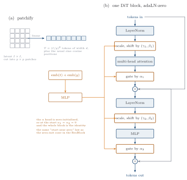
That zero-initialization is the U0.T2 “start near zero” law once more, and it is not a detail: the paper reports that adaLN-zero reaches, at 400 thousand training iterations, roughly half the FID of the in-context conditioning variant, while adding negligible cost. How the conditioning enters changes the model’s quality substantially.
One sentence on scale, and then stop. Across model sizes from 12 to 28 layers and across patch sizes, larger transformer backbones give better samples, consistently and without special handling. Why that is, and what it costs, is U5.T1.
Evaluating generative models
We can now build the models. The remaining question is how to tell whether one is good — and the honest answer is that no single number does the job, so the section is organized around what each candidate measures and what it misses.
Likelihood, and what it does not tell you
The natural score is the probability the model assigns to held-out data. Because that number scales with the dimension, it is reported per dimension and in bits.
For a model density \(p_\theta\) on \(\mathbb{R}^d\) and test data \(x \sim q\), \[ \mathrm{BPD}(\theta) \;=\; -\,\frac{1}{d \, \log 2} \; \mathbb{E}_{x \sim q}\big[ \log p_\theta(x) \big] . \tag{7}\] Lower is better. The quantity is a compression rate: it is the average number of bits per dimension needed to encode a test example under a code built from \(p_\theta\).
BPD measures coverage. A model is punished, heavily, for assigning low density anywhere the data actually lives, because \(-\log p_\theta(x)\) diverges there. That is a real virtue, and it is why likelihood remains the right score when the question is density estimation.
It is not the same as sample quality, and the gap is larger than intuition suggests (Theis, Oord, and Bethge 2016). Consider a model that draws from a good generator with probability \(1 - \varepsilon\) and from pure noise with probability \(\varepsilon\). Its log-likelihood is within \(\log \frac{1}{1-\varepsilon}\) of the good model’s — a difference that, divided by \(d\) in Equation 7, is invisible for image-sized \(d\). Its samples are garbage a fraction \(\varepsilon\) of the time. Excellent likelihood is compatible with terrible samples, because likelihood is an average over the data and the damage hides in directions the average does not weight.
There is a second, blunter limitation. For several families in the U0.T3 taxonomy the number cannot be computed at all: a VAE gives only the ELBO, a lower bound; and a GAN defines no density, so the column is not merely hard to fill but empty. Any evaluation protocol that requires likelihood cannot compare across the taxonomy.
FID
The response is to compare the two distributions — real and generated — in a feature space where distance is closer to perceptual, and to accept a summary that is computable for any model you can sample from.
The recipe has three steps. Push a large set of real samples and a set of generated samples through a fixed feature extractor. Fit a Gaussian to each set of features. Report the Fréchet distance between the two Gaussians, which for Gaussians is the 2-Wasserstein distance and has a closed form.
With \((\mu_r, \Sigma_r)\) and \((\mu_g, \Sigma_g)\) the mean and covariance of the real and generated feature sets, \[ \begin{aligned} \mathrm{FID} \;=\;& \lVert \mu_r - \mu_g \rVert^2 \\ &+ \operatorname{Tr}\!\left( \Sigma_r + \Sigma_g - 2\big(\Sigma_r \Sigma_g\big)^{1/2} \right). \end{aligned} \tag{8}\] Lower is better; the value is \(0\) exactly when the two Gaussians coincide.
The Gaussian fit is an assumption, not a fact. Equation 8 compares only the first two moments of the feature distributions. Two genuinely different distributions with matching mean and covariance receive an FID of zero.
Caveats — all three are part of the definition.
Comparable only at identical extractor, preprocessing, and sample count. An FID is not a property of a model; it is a property of a model and a measurement protocol. Two numbers produced under different protocols cannot be compared, and the failure is not subtle — see Figure 6.
The estimator is biased upward, and the bias falls like \(1/n\). The FID of a set against its own distribution is not zero. More samples always give a lower number, whatever the model.
The extractor decides what “similar” means. The standard extractor is an ImageNet classifier, whose features are shaped by that task and that data. On data unlike ImageNet the features may not encode what you care about. This course therefore uses a designated small classifier for MNIST, with pinned weights, and reserves the ImageNet extractor for CIFAR and beyond.
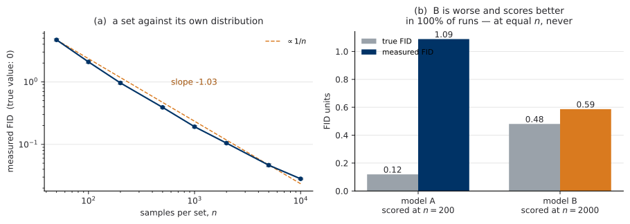
Figure 6 is worth more than the warning it replaces, because the mechanism turns out to be predictable. The left panel draws both sets from one 64-dimensional Gaussian, so the true FID is \(0\) and every point plotted is bias: about \(4.7\) at \(n = 50\), falling to \(0.028\) at \(n = 10\,000\), on a log-log slope of \(-1.03\).
The right panel takes two models, A and B, with true FIDs of \(0.12\) and \(0.48\) — B is genuinely worse by a gap of \(0.36\). Score A with \(200\) samples and B with \(2000\), and B wins in every one of 40 trials, by \(0.59\) against \(1.09\). But score them both at the same sample count, at any count tried, and the ranking is correct in every trial.
That is the whole of caveat (i), with a mechanism instead of a warning: the bias is systematic, so at equal \(n\) it lands on both models and cancels. Comparing at unequal \(n\) is what breaks it, and the ranking inverts exactly when the difference in bias exceeds the true gap. In the measured example, \(200\) against \(2000\) gives a bias difference of \(0.86\), which clears the gap of \(0.36\) and inverts always; \(500\) against \(5000\) gives \(0.34\), which misses it, and inverts in \(17.5\%\) of trials. The rule is why the harness of the next lab session logs the extractor, the preprocessing and the sample count beside every FID it returns.
Precision and recall
FID is one number, and a model can be bad in two quite different ways: it can produce unrealistic samples, or it can produce realistic samples that cover only part of the data. FID mixes both into a single score. Precision and recall separate them (Kynkäänniemi et al. 2019).
The construction is geometric. Approximate the support of each set by a union of balls: around each point, a ball whose radius reaches its \(k\)-th nearest neighbour within that same set. Then
- precision is the fraction of generated points that fall inside the real set’s support — fidelity;
- recall is the fraction of real points that fall inside the generated set’s support — coverage.
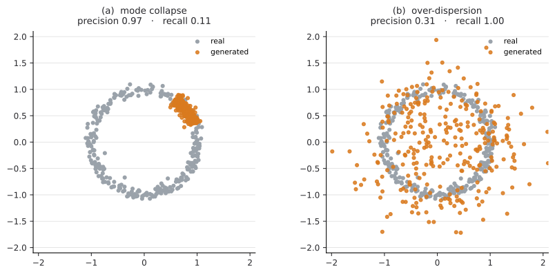
Figure 7 gives the taxonomy of U0.T3 its diagnostic vocabulary. The left panel is mode collapse, the characteristic failure of GANs: the generator produces one arc of the ring, and every sample it produces is a plausible one. It scores precision \(0.97\) and recall \(0.11\) — high fidelity, almost no coverage. The right panel is the opposite failure, an over-dispersed generator that covers the ring and a good deal of empty space besides: precision \(0.31\), recall \(1.00\).
A likelihood-trained model tends to sit at the second end, because Equation 7 punishes missing mass and is comparatively tolerant of spurious mass. This is the honest statement of the “blurry VAE samples” folklore: the blur is what covering everything looks like when the model lacks the capacity to cover it sharply.
The course treats precision and recall as a concept, not as code. The harness of the next lab session implements FID, bits per dimension and sample panels; precision and recall stay in the vocabulary, for reading papers and for naming what you see.
Where you will meet this again. U3.L2 measures the number of function evaluations against FID, and U3.L3 sweeps a conditioning strength against FID — which is where the fidelity-versus-coverage trade of this section becomes something you watch move. The harness you build in the next lab session is the instrument.
Where each part reappears
The footers of this session, collected.
| Component | Introduced | Built | Used again |
|---|---|---|---|
| Attention (Section 2) | here, once | U0.L4 (provided block) | Section 5; U5.T1; U6 seminar papers |
| U-Net anatomy (Section 3) | here | U0.L4 (unet-skeleton) |
U3.L2 first training; U3.L3; PS0 |
| Sinusoidal ladder (Equation 4) | here | U0.L4 (TODO 1) | every time-conditioned model in the course |
| FiLM / AdaGN (Equation 5) | here | U0.L4 (TODO 3) | all U3 labs; U5.T1 as adaLN |
| Embedding sum (Equation 6) | here | U0.L4 (optional pathway) | U3.L3 conditioning |
| adaLN-zero (Section 5) | preview only | — | U5.T1 |
| Bits per dimension (Equation 7) | here | U0.L4 (bpd) |
U1.L2; PS1.4 |
| FID (Equation 8) | here | U0.L4 (fid, ref_stats) |
U3.L2; U3.L3; PS0 |
| Precision / recall (Section 6.3) | here, concept only | not implemented | vocabulary for reading U6 papers |
Next session
The next lab session (U0.L4) builds two things at once, and both are components of PS0.
The first is the time-conditioned U-Net: Figure 2 assembled, with the conditioning path of Section 4 wired into every block. Its interface is frozen in that session — forward(x, t, y=None), with t a (B,) float tensor in \([0,1]\) asserted at the door — because U3 imports it unchanged.
The second is the evaluation harness: Equation 8 and Equation 7 implemented, with the caveats of Section 6.2 enforced by code rather than by memory. The harness is calibrated before it is trusted — scored against a held-out split, against a deliberately corrupted set, and against itself at several sample counts to reproduce the left panel of Figure 6 — and its first real use is to measure the VAE you trained in U0.L3.