U1.T1 — Change of Variables and Coupling Flows
Session U1.T1 · date: see calendar-map
How to read this page. This is the first content session of the joint phase, and it is where generative modeling starts. The previous session (UP.T1) ended on a debt: maximum likelihood needs \(\log p_\theta(x_1)\) at every data point, and a generative model as defined there only knows how to sample. This page pays that debt in the most direct way there is. It shows the one architectural principle that makes the log-density exactly computable, and then it shows the price.
These notes are written to be read on their own. They depend on the async primer (UP.A, in particular its §4) and on UP.T1, and on nothing else. You do not need to have attended the bootcamp. Where a bootcamp artifact is named, the thing it names is written out here in full.
Two references cover this material at book length and both are optional: (Bishop and Bishop 2024) ch. 18 (its §18.1 is the coupling-flow part of this page), and the survey (Papamakarios et al. 2021), whose §2.1 is the theorem and §3.1.2 is the coupling layer. The two original papers, (Dinh, Krueger, and Bengio 2015) and (Dinh, Sohl-Dickstein, and Bengio 2017), are short and readable, and §4 and §5 below cite them section by section.
What must \(\psi^{\theta}\) satisfy for \(\log p_\theta(x_1)\) to be exactly computable?
The live session keeps this question on the board from the first minute to the last. This page answers it in §2, sharpens it in §3, builds the answer in §4 and §5, and writes it out in one line in Section 8.1. A second question joins it in §6, and that one is not answered today.
§1 — The exact-likelihood contract
Reference for this section: UP.T1 §4, whose results are restated here without proof.
What UP.T1 left on the table
Three facts, all from UP.T1.
- A generative model is a pushforward of noise: \[ p_\theta \;=\; \big(\psi^{\theta}\big)_{\#}\, p_0 , \qquad p_0 = \mathcal{N}(0, I_d) . \tag{1}\] The source \(p_0\) is fixed. The map \(\psi^{\theta}\) is the only learned object. To sample, draw \(x_0 \sim p_0\) and return \(\psi^{\theta}(x_0)\). The time convention is the course’s: \(t = 0\) is noise, \(t = 1\) is data, so the map runs from \(x_0\) to \(x_1\).
- Maximum likelihood is a KL. With \(q\) the data distribution, \[ \operatorname*{arg\,max}_{\theta}\; \mathbb{E}_{x_1 \sim q}\big[\, \log p_\theta(x_1) \,\big] \;=\; \operatorname*{arg\,min}_{\theta}\; \mathrm{KL}\big(q \,\Vert\, p_\theta\big) . \tag{2}\]
- Therefore training needs \(\log p_\theta(x_1)\) at data points \(x_1 \sim q\), and Equation 1 does not provide it. It provides samples.
The problem, stated honestly
Take a generic neural network as \(\psi^{\theta}\), say a multilayer perceptron from \(\mathbb{R}^{d}\) to \(\mathbb{R}^{d}\). What is the density of \(\psi^{\theta}(x_0)\) at a point \(x_1\)? Formally it is an integral over every noise point that lands on \(x_1\): \[ p_\theta(x_1) \;=\; \int p_0(x_0)\; \delta\big(x_1 - \psi^{\theta}(x_0)\big)\, \mathrm{d}x_0 . \tag{3}\] For a generic map this is not computable. The set of preimages \(\{x_0 : \psi^{\theta}(x_0) = x_1\}\) has no closed form, may be empty, and may be infinite. If the network’s output lives on a lower-dimensional surface the density does not even exist. Nothing about a standard architecture prevents any of this.
Two escape routes exist. One is to give up on the exact value and settle for a lower bound on \(\log p_\theta(x_1)\). The variational autoencoder takes that route; the bootcamp session U0.T3 covered it, and nothing on this page depends on it. The other is to make the density exact by construction: restrict \(\psi^{\theta}\) to a class of maps for which Equation 3 collapses to a formula. This unit takes the second route, and the formula it collapses to is the subject of §2.
The exact-likelihood contract is the standing benchmark of the course. U2 keeps it, at the price of running a differential-equation solver inside every training step. U3 abandons it during training and recovers it afterwards, in U3.T3. Treat it as a contract now, so that each renegotiation later is a visible event and not a quiet drift.
§2 — The change-of-variables theorem
Reference for this section: UP.A §4.3 for the one-dimensional case, and (Papamakarios et al. 2021) §2.1 for the statement used here.
In one dimension, you already proved it
UP.A §4.3 stated and derived the one-dimensional case. Let \(x\) have density \(p_x\), let \(g\) be differentiable and strictly monotone, and set \(y = g(x)\). Then \[ p_y(y) \;=\; p_x\big(g^{-1}(y)\big)\, \left| \frac{\mathrm{d}\,g^{-1}}{\mathrm{d}y}(y) \right| . \tag{4}\] The derivation ran through the cumulative distribution function and the chain rule. The content is the absolute value: it measures how much \(g\) stretches or compresses the line near \(y\), and where the map stretches, the density must fall by the same factor. Probability mass is conserved; density is not. The primer’s figure and animation showed this with a sliding interval. Exercise PS1.1.8 made you compute it for \(y = \tanh(x)\), so the one-dimensional case is a fair assumption for every reader of this page.
The primer also promised that “the multivariate version is yours to prove”, and named PS1.3. This section states that version, gives its geometry, and sketches its proof with the gaps marked. Section 2.5 is the scaffold for the proof you owe.
The theorem in \(d\) dimensions
First the words. A diffeomorphism of \(\mathbb{R}^{d}\) is a map \(\psi \colon \mathbb{R}^{d} \to \mathbb{R}^{d}\) that is a bijection, is differentiable, and whose inverse is differentiable too. Its Jacobian at \(x\) is the \(d \times d\) matrix of partial derivatives, \(J_\psi(x) = \partial \psi / \partial x\), in the notation of L1 §4. The pushforward \(\psi_{\#} p\) is the distribution of \(\psi(x)\) for \(x \sim p\), as defined in UP.T1 §4.
Let \(x \sim p\) with \(p\) a density on \(\mathbb{R}^{d}\), let \(\psi\) be a diffeomorphism of \(\mathbb{R}^{d}\), and set \(y = \psi(x)\). Then \(y\) has a density, and it is \[ \begin{aligned} (\psi_{\#} p)(y) &\;=\; p\big(\psi^{-1}(y)\big)\; \big|\det J_{\psi^{-1}}(y)\big| \\[4pt] &\;=\; \frac{p(x)}{\big|\det J_{\psi}(x)\big|} \qquad\text{with } x = \psi^{-1}(y) . \end{aligned} \tag{5}\] In log form, and with the Jacobian of the forward map, \[ \begin{aligned} \log\,(\psi_{\#} p)(y) &\;=\; \log p(x) \;-\; \log\big|\det J_{\psi}(x)\big| , \\[2pt] x &\;=\; \psi^{-1}(y) . \end{aligned} \tag{6}\]
The two expressions in Equation 5 are the same statement read from the two ends of the map. They agree because the inverse function theorem gives \(J_{\psi^{-1}}(y) = J_{\psi}(x)^{-1}\) at \(x = \psi^{-1}(y)\), and the determinant of an inverse is the inverse of the determinant. UP.A’s Equation 4 is the case \(d = 1\): a \(1 \times 1\) determinant is the number itself, and \(|\mathrm{d}g^{-1}/\mathrm{d}y|\) is \(|\det J_{g^{-1}}(y)|\).
This course writes the log form with the forward Jacobian, Equation 6, and it fixes the direction of \(\psi\) once: \(\psi^{\theta}\) generates, from noise to data, as in Equation 1. Applied to the model, the theorem reads \[ \begin{aligned} \log p_\theta(x_1) &\;=\; \log p_0(x_0) \;-\; \log\big|\det J_{\psi^{\theta}}(x_0)\big| , \\[2pt] x_0 &\;=\; \big(\psi^{\theta}\big)^{-1}(x_1) . \end{aligned} \tag{7}\] Read it as a recipe. To evaluate the log-density at a data point \(x_1\): undo the map to find the noise point \(x_0\) that produced it, evaluate the source density there, and subtract the log of the volume factor the map applied on the way. UP.T1 §4 called these “both halves” of the problem. They are now one formula.
The two original papers write the map the other way. In (Dinh, Krueger, and Bengio 2015) and (Dinh, Sohl-Dickstein, and Bengio 2017), \(f\) goes from data to the latent space, and \(f\) is our \((\psi^{\theta})^{-1}\); their \(\log|\det \partial f / \partial x|\) enters with a plus sign, which is the same sign as ours once the direction is translated. The survey (Papamakarios et al. 2021) writes \(T\) for our \(\psi\) and \(u\) for our \(x_0\). When you read any of them, translate to Equation 7 first.
\(|\det J_\psi|\) is local volume distortion
Here is the picture behind Equation 5, and it is the one thing from this section to keep. Take a small cube \(C_h\) of side \(h\) around a point \(x_0\). Its volume is \(h^{d}\), and the probability mass inside it is about \(p(x_0)\, h^{d}\). Now push the cube through \(\psi\). Because \(\psi\) is differentiable, its image is, to first order, the image of the cube under the linear map \(J_\psi(x_0)\), shifted to \(\psi(x_0)\): a parallelepiped. A linear map with matrix \(A\) multiplies every volume by \(|\det A|\), so the parallelepiped has volume \(|\det J_\psi(x_0)|\, h^{d}\).
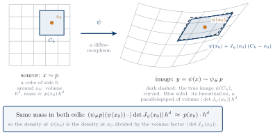
slide-volume-distortion; U2.T2 re-draws it with the cube deforming in continuous time.
Now the one physical fact: the mass does not change. Every noise point in \(C_h\) lands in \(\psi(C_h)\), and no other point does, because \(\psi\) is a bijection. So \[ \underbrace{(\psi_{\#}p)\big(\psi(x_0)\big)}_{\text{density at the image}} \;\cdot\; \underbrace{\big|\det J_\psi(x_0)\big|\, h^{d}}_{\text{volume of the image}} \;\approx\; \underbrace{p(x_0)}_{\text{density at the source}} \;\cdot\; \underbrace{h^{d}}_{\text{volume of the source}} , \] and dividing by the image volume gives the right-hand side of Equation 5. Where the map expands volume, the density drops by the same factor. Where it compresses, the density rises. The determinant is not a technicality of multivariable calculus; it is the exchange rate between volume and density.
Hold on to Figure 1. U2.T2 draws the same cube and asks how fast its volume grows as it is carried along, in continuous time. The answer there, the divergence, is the volume growth rate: the instantaneous version of the determinant here, and the picture is drawn the same way on purpose.
Proof sketch, with the gaps marked
The live session runs this argument on the board. The argument is correct in outline and has three gaps, each of which is named where it opens. PS1.3 closes all three, and the scaffold in Section 2.5 fixes the route.
Step 1 — a linear map moves volume by \(|\det A|\). For an invertible matrix \(A\) and a box \(B\), \(\mathrm{vol}(AB) = |\det A|\,\mathrm{vol}(B)\). This is what the determinant is, and it is the step everyone believes. It is also the step that needs a proof, because the definition of the determinant is a formula and the claim is about volumes. Gap 1: prove it. The route is to factor \(A\) into elementary matrices, or into orthogonal and diagonal factors, and to check each factor separately.
Step 2 — a diffeomorphism is locally linear. Differentiability at \(x_0\) says \[ \begin{aligned} \psi(x) &\;=\; \psi(x_0) + J_\psi(x_0)\,(x - x_0) + r(x), \\[2pt] \frac{|r(x)|}{|x - x_0|} &\;\to\; 0 \quad\text{as } x \to x_0 . \end{aligned} \] So for a small cube \(C_h\) at \(x_0\) the image \(\psi(C_h)\) is the parallelepiped of step 1, up to a remainder that is small compared to \(h\), and its volume is \(|\det J_\psi(x_0)|\,h^{d}\,(1 + o(1))\). Gap 2: the “\(o(1)\)” has to be controlled in a way that survives the next step. That needs the remainder to be small uniformly over a region, which is what continuity of the Jacobian provides, and it needs an argument that a small perturbation of a parallelepiped has almost the same volume.
Step 3 — mass conservation, and the limit. Because \(\psi\) is a bijection, \(\mathbb{P}[y \in \psi(C_h)] = \mathbb{P}[x \in C_h]\). Write both sides with densities, divide by \(h^{d}\), and let \(h \to 0\): \[ (\psi_{\#}p)\big(\psi(x_0)\big) \cdot \big|\det J_\psi(x_0)\big| \;=\; p(x_0) . \] Gap 3: this step assumes that \(y\) has a continuous density, which is part of what the theorem claims. The honest proof goes the other way round. It first proves the substitution rule \[ \int_{\psi(B)} g(y)\, \mathrm{d}y \;=\; \int_{B} g\big(\psi(x)\big)\, \big|\det J_\psi(x)\big|\, \mathrm{d}x \tag{8}\] for continuous \(g\) and boxes \(B\), by cutting \(B\) into small cubes, applying step 2 on each, and passing to the limit. Then it reads the density of \(y\) off Equation 8 directly. Dominated convergence is the tool for the limit, and it is the only piece of analysis the proof needs.
That is the whole argument. The three gaps are real, they are closable with first-year analysis, and closing them is the first proof-completion of the course.
PS1.3 — the multivariate change of variables
Let \(\psi\) be a diffeomorphism of \(\mathbb{R}^{d}\) with continuous Jacobian, and let \(x \sim p\) with \(p\) continuous. Prove Equation 5 along the following route. Each part closes one gap of Section 2.4.
(a) Linear maps. For an invertible \(A \in \mathbb{R}^{d \times d}\) and a box \(B = [a_1, b_1] \times \cdots \times [a_d, b_d]\), show \(\mathrm{vol}(AB) = |\det A|\,\mathrm{vol}(B)\). Hint: every invertible matrix is a product of elementary matrices (row scalings, row swaps, and row additions). Check the claim for each kind, and use \(\det(A_1 A_2) = \det A_1 \det A_2\).
(b) The local case. Fix \(x_0\) and let \(C_h\) be the cube of side \(h\) centred at \(x_0\). Show \[ \frac{\mathrm{vol}\big(\psi(C_h)\big)}{h^{d}} \;\longrightarrow\; \big|\det J_\psi(x_0)\big| \qquad (h \to 0) . \] Hint: write \(\psi(x) = \psi(x_0) + J_\psi(x_0)(x - x_0) + r(x)\). Continuity of the Jacobian gives \(|r(x)| \le \varepsilon(h)\,|x - x_0|\) on \(C_h\) with \(\varepsilon(h) \to 0\). Let \(P_h = J_\psi(x_0)(C_h - x_0)\) be the parallelepiped. Show that \(\psi(C_h) - \psi(x_0)\) is sandwiched between \((1 - c\,\varepsilon(h))\,P_h\) and \((1 + c\,\varepsilon(h))\,P_h\) for a constant \(c\) that depends only on \(\|J_\psi(x_0)^{-1}\|\), and use part (a) on the two scaled copies. (The inner inclusion is the harder one; apply the same expansion to \(\psi^{-1}\).)
(c) The global case. Fix a bounded box \(B\) and a continuous \(g \ge 0\). Cut \(B\) into cubes of side \(h\), apply part (b) on each, and pass to the limit to prove Equation 8. Hint: the sum over cubes is a Riemann sum for the right-hand side, and dominated convergence controls the error terms. State the dominating function.
(d) Read off the density. For a bounded box \(B'\) in \(y\)-space, write \(\mathbb{P}[y \in B'] = \mathbb{P}[x \in \psi^{-1}(B')]\) and apply part (c) with the map \(\psi^{-1}\) to show that \(y\) has the density in Equation 5. Finally derive Equation 6, and explain in one sentence why the forward and inverse forms of Equation 5 are the same statement.
Route fixed on purpose. Do not use measure-theoretic pushforward machinery or an appeal to “the change-of-variables formula from analysis”. The point of the exercise is to see the linearization do the work.
The fine print
Equation 5 asks three things of \(\psi\), and the live session puts them on the board without comment:
- \(\psi\) is a bijection of \(\mathbb{R}^{d}\) onto \(\mathbb{R}^{d}\);
- \(\psi\) is differentiable;
- \(\psi^{-1}\) is differentiable.
Together these say “diffeomorphism”. Each of them is a restriction on what the map is allowed to do, and each has consequences for what distributions a flow can reach. This page does not draw those consequences. It only asks you to notice that the theorem has hypotheses, and that everything built on it in §4 and §5 inherits them.
Equation 5 is used verbatim in U1.L1, where you implement it, and in PS1.4, where you book it for a three-layer model. It is generalized twice: in U2.T2, the log-determinant of a Jacobian becomes the time integral of a divergence; in U3.T3, that generalization is applied to a specific differential equation to give diffusion models a likelihood. When the Rosetta Stone gains its likelihood row in U3.T3, this theorem is the oldest ancestor in that row.
§3 — Flows are compositions, and the two costs
Reference for this section: (Papamakarios et al. 2021) §2.1 (composition) and §2.3.1 (maximum likelihood for flows).
Composition
A single diffeomorphism with a cheap Jacobian is not expressive. The way out is the way out everywhere in deep learning: stack. If \(\psi_1, \dots, \psi_K\) are diffeomorphisms, so is \[ \psi^{\theta} \;=\; \psi_K \circ \psi_{K-1} \circ \cdots \circ \psi_1 , \tag{9}\] with inverse \((\psi^{\theta})^{-1} = \psi_1^{-1} \circ \cdots \circ \psi_K^{-1}\) (the layers undone in reverse order) and, by the chain rule and \(\det(AB) = \det A \det B\), a Jacobian determinant that is the product of the layer determinants, each evaluated at the point that layer sees. The word flow refers to this chain: a sample from \(p_0\) flows through the layers to become a sample from \(p_\theta\). The word normalizing refers to the inverse direction, which carries data back to the standard source.
Name the intermediate points once, because PS1.4 books them: \[ \begin{aligned} z_0 &= x_0, \\ z_k &= \psi_k(z_{k-1}) \qquad (k = 1, \dots, K), \\ z_K &= x_1 . \end{aligned} \tag{10}\]
The log-likelihood telescopes
Apply Equation 6 to each layer of Equation 9 and add. The logs of the determinants become a sum: \[ \log p_\theta(x_1) \;=\; \log p_0(z_0) \;-\; \sum_{k=1}^{K} \log\big|\det J_{\psi_k}(z_{k-1})\big| , \tag{11}\] where the chain Equation 10 is obtained by running the inverse: start at \(z_K = x_1\) and set \(z_{k-1} = \psi_k^{-1}(z_k)\) down to \(z_0\). One line on the board, and it is the line that turns a modeling question into a design question. Every term in Equation 11 must be cheap, for every layer, at every data point, at every training step.
The two costs
A flow-based model provides two operations, and they run the map in opposite directions. Sampling runs \(\psi^{\theta}\) forward. Evaluating the density, which is what training does at every step, runs \((\psi^{\theta})^{-1}\) and needs the log-determinant of every layer on the way. UP.A §4.4 saw this tension in one dimension, where a monotone \(g\) resolves it for free. In \(d\) dimensions the two requirements pull against each other, and the whole design problem of this unit is to keep both cheap at once.
| Operation | Direction of \(\psi^{\theta}\) | Needs, per layer \(k\) | Cost driver |
|---|---|---|---|
| Sampling | forward, \(x_0 \to x_1\) | evaluate \(\psi_k\) | one pass per layer |
| Density / training (MLE) | inverse, \(x_1 \to x_0\) | evaluate \(\psi_k^{-1}\) and \(\log\lvert\det J_{\psi_k}\rvert\) | the inverse, and the log-determinant |
This table is versioned. U1.T2 adds a row per architecture (v2). U2.T2 changes what the cells contain (v3). U3.L1 shows a training method that touches neither row.
The cost driver in the second row is where a naive design dies. A dense \(d \times d\) Jacobian costs \(O(d^{2})\) to store and \(O(d^{3})\) to take the determinant of, per layer, per data point, per step. For a \(32 \times 32\) colour image \(d = 3072\), and \(d^{3} \approx 3 \times 10^{10}\). That is not slow. It is dead on arrival. And the inverse of a generic network is not available at all.
The whole architectural zoo of this unit is a list of tricks to make both rows cheap simultaneously. That sentence is the unit’s thesis. Section 4 and Section 5 give the first two entries in the zoo, and they share one idea.
Table 1 is the reading key for U1.T2, where every architecture is placed in a corner of it. It is also the precise statement of what U2 breaks (the log-determinant becomes the solution of a differential equation, and the inverse becomes the same equation run backwards) and what U3 escapes (training touches neither row).
§4 — NICE: additive coupling
Reference for this section: (Dinh, Krueger, and Bengio 2015) §3.2 (the coupling layer) and §3.3 (the scaling layer).
Split the coordinates
One remark on notation before the layer. Inside a single layer this section writes \(x\) for the input and \(y\) for the output. In the chain Equation 10 those are \(z_{k-1}\) and \(z_k\); the per-layer letters exist so that the layer can be read on its own. And when individual coordinates must be named, this page writes the halves \(x_A, x_B\) or, for a generic vector, \(\xi = (\xi_1, \dots, \xi_d)\); the symbol \(x_1\) is never a coordinate here, because L1 §4 reserves it for the data point.
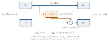
Partition the \(d\) coordinates into two blocks, \(x = (x_A, x_B)\) with \(d_A + d_B = d\). Take any function \(m_\theta \colon \mathbb{R}^{d_A} \to \mathbb{R}^{d_B}\), a neural network of your choice, and define one layer in the generative direction as follows.
\[ y_A \;=\; x_A , \qquad y_B \;=\; x_B + m_\theta(x_A) . \tag{12}\]
The first block passes through untouched. The second block is shifted by an amount that depends on the first block only. This is the additive coupling layer of NICE, and Figure 2 is Equation 12 drawn.
The Jacobian, on the board
Order the coordinates as \((x_A, x_B)\) and differentiate Equation 12 block by block: \[ J_\psi(x) \;=\; \begin{bmatrix} \dfrac{\partial y_A}{\partial x_A} & \dfrac{\partial y_A}{\partial x_B} \\[8pt] \dfrac{\partial y_B}{\partial x_A} & \dfrac{\partial y_B}{\partial x_B} \end{bmatrix} \;=\; \begin{bmatrix} I_{d_A} & 0 \\[4pt] \dfrac{\partial m_\theta}{\partial x_A}(x_A) & I_{d_B} \end{bmatrix} . \tag{13}\] The matrix is block lower-triangular, and the determinant of a block-triangular matrix is the product of the determinants of its diagonal blocks. Both diagonal blocks are identities, so \[ \det J_\psi(x) \;=\; 1 \qquad\text{and}\qquad \log\big|\det J_\psi(x)\big| \;=\; 0 . \tag{14}\] The lower-left block is the Jacobian of a neural network, which is the one expensive object in the picture, and it never enters the determinant.
The inverse is a subtraction: \[ x_A \;=\; y_A , \qquad x_B \;=\; y_B - m_\theta(y_A) . \tag{15}\] It costs exactly one forward evaluation of \(m_\theta\), the same as the forward direction. Both rows of Table 1 are as cheap as they can be.
The trick the whole family rides on
Look at Equation 15 once more. To undo the layer you evaluate \(m_\theta\) at \(y_A\), which you have, because \(y_A = x_A\). You never invert \(m_\theta\), and you never need to. Invertibility of the whole does not require invertibility of the parts. The conditioner \(m_\theta\) can be as deep, as wide, and as non-invertible as you like: a rectified network, a convolutional network, anything with the right input and output sizes. Every coupling architecture in this unit rides on this one observation.
The honest limitation
Equation 14 is too good. A layer with \(\det J \equiv 1\) preserves volume: it moves mass around but can never concentrate it or spread it. A stack of such layers preserves volume too, since the determinants multiply. So a pure additive-coupling flow can only reach distributions with the same “spread” as the source, and a real dataset does not oblige. NICE’s own fix (Dinh, Krueger, and Bengio 2015, sec. 3.3) is a final diagonal scaling layer, \(y_i = S_{ii}\, x_i\), with \(\log|\det J_\psi(x)| = \sum_i \log|S_{ii}|\) (Exercise 2 below). That layer rescales each coordinate once, globally. The next section makes the rescaling local, and that is the whole difference between NICE and RealNVP.
§5 — RealNVP: affine coupling
Reference for this section: (Dinh, Sohl-Dickstein, and Bengio 2017) §3.2 (the layer) and §3.3 (its properties).
Edit one block
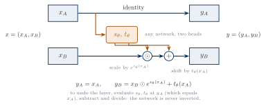
Keep the split and the pass-through half. Replace the shift by a shift and a scale, both read off \(x_A\).
\[ y_A \;=\; x_A , \qquad y_B \;=\; x_B \odot \exp\!\big(s_\theta(x_A)\big) + t_\theta(x_A) , \tag{16}\]
Here \(s_\theta, t_\theta \colon \mathbb{R}^{d_A} \to \mathbb{R}^{d_B}\) are arbitrary networks (in practice one network with two output heads) and \(\odot\) is the elementwise product. The exponential keeps every scale positive, so each coordinate of \(x_B\) is stretched or compressed but never flipped or collapsed. This is the affine coupling layer of RealNVP.
The Jacobian, edited in place
The board plan of the live session derives NICE’s Jacobian first and then edits it, in place, into RealNVP’s. The edit is one block.
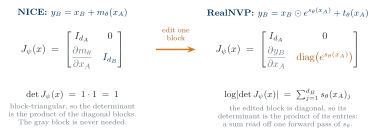
In symbols, \[ \begin{aligned} J_\psi(x) &\;=\; \begin{bmatrix} I_{d_A} & 0 \\[4pt] \dfrac{\partial y_B}{\partial x_A} & \operatorname{diag}\!\big(e^{s_\theta(x_A)}\big) \end{bmatrix} , \\[6pt] \log\big|\det J_\psi(x)\big| &\;=\; \sum_{j=1}^{d_B} s_\theta(x_A)_j . \end{aligned} \tag{17}\] Block lower-triangular again, so the determinant is the product of the diagonal blocks; the first is \(1\), and the second is the product of the diagonal entries \(e^{s_\theta(x_A)_j}\). The log turns that product into a sum. The log-determinant is a sum read off a forward pass of \(s_\theta\). No \(d \times d\) matrix is ever formed, and no determinant is ever computed.
The inverse is a subtraction and a division: \[ x_A \;=\; y_A , \qquad x_B \;=\; \big(y_B - t_\theta(y_A)\big) \odot \exp\!\big(-s_\theta(y_A)\big) . \tag{18}\] As with NICE, \(s_\theta\) and \(t_\theta\) are evaluated at \(y_A = x_A\) and never inverted, and the cost of the inverse equals the cost of the forward pass.
One consequence is worth saying out loud because U1.L1 uses it. The log-determinant Equation 17 depends on \(x_A\) only, and \(x_A = y_A\) is available on both sides of the layer. So the sum \(\sum_j s_\theta(\cdot)_j\) can be read during the inverse pass, which is the pass training runs, with no extra work. Exercise 3 checks the sign.
NICE and RealNVP, side by side
The live session obtains RealNVP’s Jacobian by editing NICE’s in place, and the edit is the pedagogy. Here is the static record of it, one row per property.
| NICE (additive) | RealNVP (affine) | |
|---|---|---|
| Layer | \(y_B = x_B + m_\theta(x_A)\) | \(y_B = x_B \odot e^{s_\theta(x_A)} + t_\theta(x_A)\) |
| \(\log\lvert\det J_\psi\rvert\) | \(0\) | \(\sum_j s_\theta(x_A)_j\) |
| Inverse | subtract; one pass of \(m_\theta\) | subtract, then divide; one pass of \(s_\theta, t_\theta\) |
| Volume | preserved; NICE adds a global scaling layer | changed locally, per layer |
| Untouched half | \(x_A\), read by the conditioner | \(x_A\), read by the conditioner |
In both columns, both rows of Table 1 cost one conditioner pass per layer, in both directions. That is the design achievement, and RealNVP adds the local volume change without giving any of it up.
What one layer does to a grid
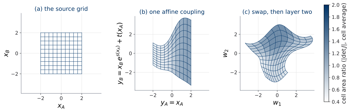
Panel (b) of Figure 5 is Equation 17 made visible. The Jacobian determinant of a coupling layer is a function of the untouched half only, so the volume factor is constant along every line of constant \(x_A\). Panel (c) is §6 in advance: a single layer leaves half the coordinates alone, and it takes a permutation and a second layer to move all of them.
A numerical aside, for the lab
The exponential in Equation 16 is a liability in floating point. If \(s_\theta\) outputs a large positive number, \(e^{s}\) overflows (single precision gives up near \(s \approx 88\)); a large negative number makes the inverse Equation 18 divide by a number near zero. Early in training, when \(s_\theta\) is a random network, both happen. Implementations therefore bound the scale: a common choice passes the raw output through a \(\tanh\), scaled by a learned or fixed constant, before exponentiation. (The paper does not prescribe this; it is implementation practice.) The lab (U1.L1) makes this concrete, including what the loss curve looks like when you forget. One paragraph here is enough.
The training loss, in full
Put Equation 11 inside the maximum-likelihood objective Equation 2. With \(K\) affine coupling layers and the chain Equation 10, the loss this course minimizes is \[ \begin{aligned} \mathcal{L}(\theta) &\;=\; -\;\mathbb{E}_{x_1 \sim q}\Big[\, \log p_0\big(z_0\big) \\[2pt] &\qquad\qquad\quad \;-\; \sum_{k=1}^{K} \log\big|\det J_{\psi_k}(z_{k-1})\big| \,\Big] , \\[4pt] &\phantom{\;=\;} z_K = x_1,\qquad z_{k-1} = \psi_k^{-1}(z_k) . \end{aligned} \tag{19}\] Every symbol in it is now concrete. The expectation is over data, and the subscript says so; the primer’s §5 made that mandatory and this is the first loss of the course where it is enforced. The chain is the inverse pass. Each log-determinant is a sum of scales, Equation 17, evaluated at the untouched half of the corresponding intermediate point. And \(\log p_0(z_0) = -\tfrac12\|z_0\|^{2} - \tfrac{d}{2}\log 2\pi\) is the standard Gaussian, in closed form.
Let \(d = 4\), and write the coordinates of any vector \(\xi \in \mathbb{R}^{4}\) as \((\xi_1, \xi_2, \xi_3, \xi_4)\) (the letter \(x\) is not used for coordinates here, because \(x_1\) is the data point). Let \(\psi^{\theta} = \psi_3 \circ \psi_2 \circ \psi_1\) where each \(\psi_k\) is an affine coupling layer Equation 16 with its own conditioner networks \(s^{(k)}, t^{(k)}\), and the splits alternate: \(\psi_1\) and \(\psi_3\) condition on the first two coordinates \((\xi_1, \xi_2)\) and move the last two \((\xi_3, \xi_4)\); \(\psi_2\) conditions on \((\xi_3, \xi_4)\) and moves \((\xi_1, \xi_2)\).
(a) Write out the inverse pass Equation 10 for a data point \(x_1 \in \mathbb{R}^{4}\): give \(z_2\), \(z_1\), \(z_0\) explicitly in terms of the conditioners, in the order they are computed.
(b) Write \(\log p_\theta(x_1)\) for this model as a fully explicit expression, with every \(\log|\det J_{\psi_k}|\) replaced by its sum of scales and every scale evaluated at the correct intermediate point. State which half of which \(z_k\) each conditioner reads.
(c) Write the loss Equation 19 for a minibatch of \(B\) data points, with the expectation replaced by the sample mean and the sampling subscript kept.
(d) Suppose \(\psi_2\) is replaced by a swap of the two halves, \((\xi_1, \xi_2, \xi_3, \xi_4) \mapsto (\xi_3, \xi_4, \xi_1, \xi_2)\). Redo part (b). Which term changes, and what is the new log-determinant of the middle layer?
This exercise is mechanical on purpose. It forces the notation of Equation 19 through your hands once, before U1.L1 forces it through code.
§6 — Masks, partitions, and permutations
Reference for this section: (Dinh, Sohl-Dickstein, and Bengio 2017) §3.4 and §3.5, and (Dinh, Krueger, and Bengio 2015) §3.2 (“combining coupling layers”).
\(x_A\) is never touched, so alternate
A coupling layer leaves \(x_A\) exactly as it found it. A stack of layers that all use the same split leaves \(x_A\) alone forever, and the model is a distribution on \(x_B\) only. Two standard remedies:
- Alternate the split. Layer \(k\) conditions on block \(A\) and moves block \(B\); layer \(k+1\) conditions on \(B\) and moves \(A\). After two layers every coordinate has moved, and after three every coordinate has been able to influence every other, which is the smallest depth at which the composed Jacobian can be dense (Dinh, Krueger, and Bengio 2015, sec. 3.2).
- Permute between layers. Keep one split and insert a fixed permutation of the coordinates between coupling layers. A permutation is a linear map with matrix \(P\); it is a bijection, its inverse is \(P^{\top}\), and \(|\det P| = 1\), so its contribution to Equation 11 is zero. Exercise 1 asks you to check this in your head now; U1.L1 asks you to check it in code.
For images, RealNVP writes the split as a binary mask \(b\) over pixels and channels, \(y = b \odot x + (1 - b) \odot \big(x \odot e^{s(b \odot x)} + t(b \odot x)\big)\), with checkerboard and channel-wise patterns (Dinh, Sohl-Dickstein, and Bengio 2017, sec. 3.4). That is U1.L2 material, and one line is all it gets here.
Depth as the lever
With alternation or permutations in place, a stack of \(K\) affine coupling layers moves every coordinate, and the Jacobian of the composition is dense once \(K \ge 3\). The natural next belief is that depth buys expressivity: that with enough layers, a coupling flow can push \(\mathcal{N}(0, I_d)\) onto anything. This page asserts that depth is the lever and does not prove it. The live session writes a second question on the board, next to the session question:
How expressive is a stack of these, really?
Posed today. Answered in U1.T2, which is where the fine print of Section 2.6 comes back.
§7 — Training by maximum likelihood
Reference for this section: (Papamakarios et al. 2021) §2.3.1.
The loop, in full
Training a flow is ordinary supervised-style optimization with a specific loss. Nothing about the loop is specific to flows; only the loss line is. Here is the whole loop, so that this page depends on no earlier lab.
for x1 in loader:                      # a minibatch, x1 ~ q
    loss = -flow_log_prob(x1).mean()   # minus the mean of log p_theta(x1)
    opt.zero_grad()
    loss.backward()
    opt.step()
    sched.step()
flow_log_prob(x1) is Equation 11: run the inverse chain Equation 10 from \(z_K = x_1\) down to \(z_0\), add \(\log p_0(z_0)\) and subtract the \(K\) sums of scales Equation 17 on the way. You write it next session (U1.L1). opt is AdamW at base learning rate \(3 \times 10^{-4}\) with weight decay \(0.01\); sched is a linear warmup over the first few percent of steps followed by cosine decay. Those are the course’s standing defaults.
For readers of the bootcamp: this is training-loop-template with the loss line swapped, run under optimizer-schedule-defaults (the U0.T2 recipe card). For everyone else: the box above is the definition, and it is complete.
Every training step runs the inverse of every layer and reads \(K\) sums of scales. The cost per step is therefore \(K\) conditioner evaluations, exactly the cost of sampling. That symmetry is the design achievement of the coupling layer, and it is what Table 1 asks for. It is also what U2 gives up, and the reason U2’s labs are slow.
§8 — Exercises, with answers
Work these before reading the answers. Each one is a claim made on this page without proof.
Exercise 1 — permutations are free
Let \(P\) be a \(d \times d\) permutation matrix and \(\psi(x) = Px\). Show that \(\psi\) is a diffeomorphism, give its inverse, and show that its contribution to Equation 11 is zero.
\(\psi\) is linear and \(P\) is invertible, so \(\psi\) is a bijection, and both \(\psi\) and \(\psi^{-1}\) are linear, hence differentiable. A permutation matrix is orthogonal, \(P^{\top}P = I\), so \(\psi^{-1}(y) = P^{\top} y\). The Jacobian is \(J_\psi(x) = P\) at every \(x\), and \(\det P = \pm 1\) (a permutation matrix is obtained from \(I\) by row swaps, each of which flips the sign of the determinant). So \(|\det P| = 1\) and \(\log|\det J_\psi| = 0\): a permutation layer adds nothing to the sum in Equation 11, and costs nothing to invert.
Exercise 2 — NICE’s scaling layer
Let \(\psi(x) = \operatorname{diag}(e^{\sigma})\, x\) with \(\sigma \in \mathbb{R}^{d}\) a learned vector. Give the inverse and the log-determinant, and explain in one sentence why NICE needs this layer and RealNVP does not.
The map scales coordinate \(i\) by \(e^{\sigma_i} > 0\). Its inverse scales by \(e^{-\sigma_i}\). The Jacobian is the diagonal matrix itself, so \(\log|\det J_\psi| = \sum_{i=1}^{d} \sigma_i\), the same at every \(x\). NICE needs it because every additive coupling layer has \(\det J = 1\), so the stack cannot change volume at all, and a data distribution with a different spread from the source is unreachable without a global rescaling. RealNVP’s affine layer already rescales, locally and per layer, through \(e^{s_\theta(x_A)}\); a global scaling layer is then redundant, though harmless. (NICE writes the scale as \(S_{ii}\) directly; writing it as \(e^{\sigma_i}\) is the same layer with the sign taken care of.)
Exercise 3 — the Jacobian of the inverse coupling layer
Compute the Jacobian of the inverse affine coupling layer Equation 18, as a map from \(y\) to \(x\), in block form. Give its log-determinant, and say which half of \(y\) it is evaluated at.
Differentiate Equation 18 with the coordinates ordered \((y_A, y_B)\): \[ J_{\psi^{-1}}(y) \;=\; \begin{bmatrix} I_{d_A} & 0 \\[4pt] \dfrac{\partial x_B}{\partial y_A} & \operatorname{diag}\!\big(e^{-s_\theta(y_A)}\big) \end{bmatrix} , \qquad \log\big|\det J_{\psi^{-1}}(y)\big| \;=\; -\sum_{j=1}^{d_B} s_\theta(y_A)_j . \] Block lower-triangular again, with the lower-right block the elementwise inverse of the forward one. The log-determinant is minus the forward sum, and it is evaluated at \(y_A\), which equals \(x_A\). This is the identity \(\det J_{\psi^{-1}}(y) = 1 / \det J_\psi(x)\) from Section 2.2, verified by hand on one layer, and it is why the inverse pass can read the sum in Equation 19 with no extra computation.
Exercise 4 — the shading in Figure 5
Take the layer of Figure 5(b): \(y_A = x_A\), \(y_B = x_B\, e^{s(x_A)} + t(x_A)\). Show that the image of the rectangle \([a, b] \times [c, c']\) in the \((x_A, x_B)\) plane has area \((c' - c) \int_a^b e^{s(x_A)}\, \mathrm{d}x_A\), exactly, and conclude that the area ratio is the average of \(e^{s}\) over \([a, b]\) and is independent of \(c\) and \(c'\).
Apply Equation 8 with \(g \equiv 1\) and \(B = [a, b] \times [c, c']\). The Jacobian determinant of the layer is \(e^{s(x_A)}\), by Equation 17 with \(d_B = 1\). So \[ \mathrm{area}\big(\psi(B)\big) \;=\; \int_a^b\!\!\int_c^{c'} e^{s(x_A)}\, \mathrm{d}x_B\, \mathrm{d}x_A \;=\; (c' - c) \int_a^b e^{s(x_A)}\, \mathrm{d}x_A . \] Dividing by the source area \((b - a)(c' - c)\) leaves the average of \(e^{s}\) over \([a, b]\), which does not depend on \(c\) or \(c'\). That is why every cell in a column of Figure 5(b) has the same shade. The figure script computes the polygon areas numerically and checks them against this average before drawing; the worst disagreement is \(5 \times 10^{-8}\).
Reading the board
The live session closes by reading its board. Here is the same reading.
| On the board | Status |
|---|---|
| The session question — what must \(\psi^{\theta}\) satisfy for \(\log p_\theta(x_1)\) to be exactly computable? | Answered. \(\psi^{\theta}\) must be a diffeomorphism (Section 2.6), built from layers whose inverse and log-determinant are both cheap (Table 1). Coupling layers (§4, §5) are the first family that satisfies both. |
| The depth question — how expressive is a stack of these? | Open. U1.T2. |
| The fine print — bijection, differentiable, both ways | Unexamined. U1.T2. |
Where this page reappears
| From this page | Reappears in |
|---|---|
| The change-of-variables theorem, Equation 5 and Equation 6 | U1.L1 (implemented); PS1.3 (proved); U2.T2 (generalized); U3.T3 (applied to diffusion) |
| The volume picture, Figure 1 | U2.T2, re-drawn in continuous time |
| The telescoped log-likelihood, Equation 11 | PS1.4; every flow lab |
| The two costs, Table 1 | U1.T2 (v2, the zoo placed in it); U2.T1 and U2.T2 (v3, the table breaks); U3.L1 (irrelevant by design) |
| The coupling trick of Section 4.3 | U1.L1 (coupling-layer-scratch); U1.L2 |
| The fine print, Section 2.6, and the depth question | U1.T2 |
| The loss Equation 19, fully subscripted | every loss in the course, by the same rule |
Next session
The next session is the lab (U1.L1). You implement an affine coupling layer and a permutation from scratch, check the sum of scales against an automatic-differentiation Jacobian, and train the result on two-dimensional toy data by the loop of Section 7.1. The theory session after it (U1.T2) opens the rest of the zoo, and answers the depth question.
Before then: PS1.3 (Section 2.5) and PS1.4 (Section 5.6) are assigned today.