U0.T1 — Supervised Learning and Autodiff
Session U0.T1 · date: see calendar-map
These notes accompany the course opener. Two jobs today: (1) establish the ERM/MLE frame that every later loss in this course instantiates, and (2) present backpropagation as reverse-mode automatic differentiation on computational graphs, so that when the adjoint method arrives in U2.T1 it lands as “backprop through time, continuous limit” rather than as a new idea.
A word on course culture, since this is day one. Three rules of the house: every core object gets implemented from scratch at least once (libraries are cross-checks, never substitutes); notation is law — there is a course-wide standard, and its first rule is enforced from the first formula below: no loss without explicit sampling subscripts on \(\mathbb{E}\); and proofs come in two kinds, live (one today, in the VJP section below) and assigned (proof-completions in problem sets, starting in PS1). Standing references for this unit: (Bishop and Bishop 2024; Murphy 2023).
ERM and the MLE view
We want a machine that predicts \(y\) from \(x\). Before any formalism, that requires saying what counts as good prediction, on average over what. The “over what” is the data distribution — and we install its course-wide symbol immediately.
Data pairs \((x, y) \sim q\), a distribution on \(\mathbb{R}^d \times \mathcal{Y}\); a hypothesis \(f_\theta : \mathbb{R}^d \to \mathcal{Y}\) with parameters \(\theta \in \mathbb{R}^p\); and a loss \(\ell(\hat{y}, y) \ge 0\) scoring the prediction \(\hat{y} = f_\theta(x)\) against the observed \(y\).
The symbol \(q\) is this course’s name for the data distribution, here and everywhere: when we reach generative modeling, the model’s entire job will be to become \(q\). Getting used to it in the supervised setting costs nothing and pays later.
The risk and the empirical risk of \(\theta\) are \[ R(\theta) \;=\; \mathbb{E}_{(x,y)\sim q}\!\left[\, \ell\big(f_\theta(x),\, y\big) \right], \qquad \widehat{R}_n(\theta) \;=\; \frac{1}{n} \sum_{i=1}^{n} \ell\big(f_\theta(x_i),\, y_i\big), \] where \((x_i, y_i) \overset{\text{iid}}{\sim} q\) is the training set. Empirical risk minimization (ERM) is the program \(\min_\theta \widehat{R}_n(\theta)\).
Note the subscript on the expectation. It is not decoration: in this course a loss written without its sampling subscripts is considered ill-formed. Every loss we will ever write states explicitly what is sampled from where — the habit is cheap here, where there is only one distribution in sight, and essential later, when a single loss samples time, data, and a conditional path in one expectation.
Maximum likelihood is ERM with a specific loss
Choose a probabilistic model: a conditional density \(p_\theta(y \mid x)\). Take the loss to be the negative log-likelihood (NLL), \[ \ell\big(f_\theta(x),\, y\big) \;=\; -\log p_\theta(y \mid x). \] Then empirical risk minimization is exactly maximum likelihood on the dataset: \[ \min_\theta \; \frac{1}{n}\sum_{i=1}^{n} -\log p_\theta(y_i \mid x_i) \;=\; \max_\theta \; \log \prod_{i=1}^{n} p_\theta(y_i \mid x_i) \;=\; \max_\theta \; \prod_{i=1}^{n} p_\theta(y_i \mid x_i), \] since \(\log\) is monotone. The familiar losses of deep learning are not ad hoc scoring rules — each is the NLL of a specific noise model. We derive the two canonical cases in full.
Model the observation as the network’s prediction plus Gaussian noise: \[ p_\theta(y \mid x) \;=\; N\!\big(y;\, f_\theta(x),\, \sigma^2 I_k\big), \qquad y \in \mathbb{R}^k,\; \sigma^2 \text{ fixed}. \] Written out, the Gaussian density is \[ p_\theta(y \mid x) \;=\; \big(2\pi\sigma^2\big)^{-k/2} \exp\!\Big( -\tfrac{1}{2\sigma^2}\, \big\lVert y - f_\theta(x)\big\rVert^2 \Big). \] Taking the negative logarithm, \[ -\log p_\theta(y \mid x) \;=\; \frac{1}{2\sigma^2}\,\big\lVert y - f_\theta(x)\big\rVert^2 \;+\; \frac{k}{2}\,\log\!\big(2\pi\sigma^2\big). \] The second term does not depend on \(\theta\), and the prefactor \(1/2\sigma^2\) is a positive constant, so \[ \arg\min_\theta\; \mathbb{E}_{(x,y)\sim q}\big[ -\log p_\theta(y \mid x) \big] \;=\; \arg\min_\theta\; \mathbb{E}_{(x,y)\sim q}\big\lVert y - f_\theta(x)\big\rVert^{2}. \] Mean squared error is maximum likelihood under a Gaussian noise model. Four lines.
For classification into \(C\) classes, let the network output a probability vector via softmax: \(\pi(x; \theta) \in \Delta^{C-1}\) with components \(\pi_c(x;\theta) > 0\), \(\sum_c \pi_c = 1\). The categorical model is \[ p_\theta(y \mid x) \;=\; \prod_{c=1}^{C} \pi_c(x;\theta)^{\,\mathbb{1}[y = c]} \;=\; \pi_y(x;\theta). \] Hence \[ -\log p_\theta(y \mid x) \;=\; -\sum_{c=1}^{C} \mathbb{1}[y = c]\, \log \pi_c(x;\theta) \;=\; -\log \pi_y(x;\theta), \] which is the cross-entropy between the one-hot encoding of \(y\) and the predicted distribution \(\pi(x;\theta)\). (On the slides this was stated only; this is the full derivation.)
Since the names “cross-entropy” and “KL” carry the weight of the whole MLE story, we fix their definitions here once.
\[ \mathrm{KL}(p \,\|\, q) \;=\; \mathbb{E}_{x\sim p}\!\left[ \log \frac{p(x)}{q(x)} \right] \;\ge\; 0, \qquad \text{with equality iff } p = q. \]
\[ \begin{aligned} H(p, q) &\;=\; -\,\mathbb{E}_{x\sim p}\big[\log q(x)\big] \;=\; H(p) + \mathrm{KL}(p \,\|\, q), \\[2pt] H(p) &\;=\; -\,\mathbb{E}_{x\sim p}\big[\log p(x)\big]. \end{aligned} \]
The entropy \(H(p)\) does not depend on the second argument, so minimizing cross-entropy and minimizing KL in the second slot are the same problem. In particular, today’s loss \(\mathbb{E}_{(x,y)\sim q}\big[-\log p_\theta(y \mid x)\big]\) is exactly a cross-entropy — the data distribution in the sampling slot, the model inside the log — which is the MLE \(\Leftrightarrow\) KL bridge that UP.T1 proves properly.
MLE \(\Leftrightarrow\) KL minimization is proved properly in UP.T1; flows (U1) are trained by exactly this template with log-likelihood made tractable by the change of variables.
And the sentence to keep for the whole course:
“Much of this course is about what to do when the model’s likelihood is easy to sample but hard to evaluate — or vice versa.”
Normalizing flows (U1) will make the likelihood evaluable at an architectural price; Flow Matching (U3) will sidestep likelihood evaluation during training altogether. Both moves are responses to exactly this tension.
Loss surfaces and generalization, honestly
Two topics that a longer course would spend weeks on; we spend one section, deliberately, and say clearly what we are not doing.
The loss surface. For a neural network, \(\widehat{R}_n(\theta)\) is non-convex in \(\theta\), and no optimizer we use comes with a global-optimality certificate. The empirical facts: overparameterized networks train reliably to near-zero training loss with standard recipes (gradient methods such as SGD — recipes are U0.T2’s topic), and “flat minima generalize better” is folklore — suggestive intuition, not a load-bearing result. We flag it as such and move on.
Generalization. The classical bias–variance picture predicts a U-shaped test risk in model capacity; modern overparameterized practice exhibits double descent — test risk peaks near the interpolation threshold and descends again beyond it.
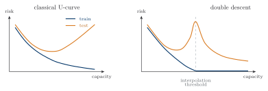
Our working answer to “will it generalize?” is not theory but experimental hygiene — proper train/val/test splits, honest evaluation, seeds and logging — built as a reusable stack in U0.L2. Why this matters later: generative models are trained by the same optimizers on the same kind of surfaces; nothing beyond this section’s honesty and that lab’s hygiene will be needed.
MLPs and universal approximation
An MLP with \(L\) layers is the composition \[ \begin{aligned} x^{0} &= x, \qquad x^{k} = \sigma\big(W_k\, x^{k-1} + b_k\big) \quad (k = 1, \dots, L-1), \\[2pt] f_\theta(x) &= W_L\, x^{L-1} + b_L, \end{aligned} \] with parameters \(\theta = \{W_k, b_k\}_{k=1}^{L}\) and \(\sigma\) an elementwise activation function.
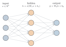
On activations: the ReLU family carries the intuition (piecewise-linear, cheap, sparse gradients); the smooth variants SiLU and GELU are what we will actually use in the U-Nets and DiT blocks from U0.T4 onward. Nothing today depends on the choice.
What can such functions represent? The classical answer:
Let \(\sigma : \mathbb{R} \to \mathbb{R}\) be continuous and non-polynomial, and let \(K \subset \mathbb{R}^d\) be compact. Then the set of one-hidden-layer networks \[ \Big\{\, x \mapsto \textstyle\sum_{j=1}^{N} a_j\, \sigma\big(w_j^{\top} x + b_j\big) \;:\; N \in \mathbb{N},\; a_j, b_j \in \mathbb{R},\; w_j \in \mathbb{R}^d \,\Big\} \] is dense in \(C(K)\) with respect to the sup norm: for every continuous \(f : K \to \mathbb{R}\) and \(\varepsilon > 0\) there is a network \(g\) in the set with \(\sup_{x \in K} |f(x) - g(x)| < \varepsilon\).
Statement only — we will not prove it, and we record two caveats with the same emphasis as the theorem. (i) It says nothing about learnability: it asserts the existence of a good network, not that any algorithm — least of all gradient descent on \(\widehat{R}_n\) — will find it. (ii) It is silent on cost: the width \(N\) needed for a given \(\varepsilon\) may be astronomically large, and width/depth tradeoffs are not quantified here. Classical sources: Cybenko (1989) and Hornik (1991); for textbook treatments, the MLP chapters of Bishop and Bishop (2024) and the corresponding parts of Murphy (2023) are the course’s standing references.
In U1.T2 we meet universality questions again for invertible models — where the answer is subtler because invertibility is a real constraint. Keep today’s fine print in mind.
The last structural observation sets up everything that follows: an MLP is a composition, \(f_\theta = f_L \circ f_{L-1} \circ \cdots \circ f_1\). Training by gradient descent needs derivatives of long compositions, cheaply and mechanically. That is a question about computational graphs.
Computational graphs and VJPs
A numerical program is usefully viewed as a computational graph: nodes are primitive operations (matrix multiply, addition, elementwise \(\sigma\), …), edges carry data. Evaluating a loss \(\mathcal{L}(\theta)\) runs the graph forward and — this detail is the crux of the whole section — caches the intermediate values \(x^{1}, x^{2}, \dots\) at every node.
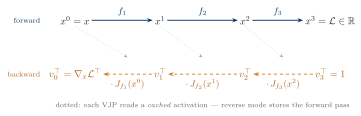
Differentiation is then another pass over the same graph. The only questions are the direction of the pass and its cost — and the right primitive to reason with is not “the gradient of everything” but the vector–Jacobian product.
Let \(f : \mathbb{R}^n \to \mathbb{R}^m\) be differentiable at \(x\), with Jacobian \(J_f(x) = \partial f / \partial x \in \mathbb{R}^{m \times n}\). For a cotangent row vector \(v^{\top} \in \mathbb{R}^{1 \times m}\), the vector–Jacobian product (VJP) of \(f\) at \(x\) is \[ \mathrm{VJP}_f(v;\, x) \;=\; v^{\top} J_f(x) \;\in\; \mathbb{R}^{1 \times n}. \]
Two remarks, both load-bearing. First, the row-vector discipline is deliberate: cotangents are linear functionals on outputs, and keeping them as rows makes the composition rule below a one-liner. Second, for every primitive used in deep learning, \(v^{\top} J_f(x)\) is computable at roughly the cost of one forward evaluation of \(f\), without ever materializing \(J_f(x)\) — e.g., for \(f(x) = W x\) the VJP is \(v^{\top} W\), one matrix–vector product, not a stored \(m \times n\) Jacobian. This is the fact that makes reverse mode \(O(1\ \text{forward-cost})\) per scalar output.
The session’s live proof is the composition rule — boxed and numbered, because U2.T1 will cite it by name.
Let \(f : \mathbb{R}^n \to \mathbb{R}^m\) be differentiable at \(x\) and \(g : \mathbb{R}^m \to \mathbb{R}^p\) differentiable at \(f(x)\), and set \(h = g \circ f\). Then, by the chain rule, \(J_h(x) = J_g(f(x))\, J_f(x)\), and for every cotangent \(v^{\top} \in \mathbb{R}^{1\times p}\): \[ \begin{aligned} v^{\top} J_h(x) &\;=\; \big(v^{\top} J_g(f(x))\big)\, J_f(x), \\[4pt] \text{i.e.}\qquad \mathrm{VJP}_h(v;\, x) &\;=\; \mathrm{VJP}_f\big(\, \mathrm{VJP}_g(v;\, f(x));\; x \,\big). \end{aligned} \] More generally, for \(h = f_L \circ \cdots \circ f_1\) with intermediates \(x^{k} = f_k(x^{k-1})\), \(x^{0} = x\), define \[ v_L^{\top} \;=\; v^{\top}, \qquad v_{k-1}^{\top} \;=\; v_k^{\top}\, J_{f_k}\big(x^{k-1}\big) \quad (k = L, \dots, 1). \] Then \(v_0^{\top} = v^{\top} J_h(x)\): reverse-mode differentiation is right-to-left accumulation of VJPs along the graph.
Proof. Two maps. Matrix multiplication is associative, so \(v^{\top}\big(J_g(f(x))\, J_f(x)\big) = \big(v^{\top} J_g(f(x))\big) J_f(x)\). The content is in the reading order: the left-hand side first forms the product \(J_g J_f \in \mathbb{R}^{p \times n}\) at cost \(O(p\,m\,n)\); the right-hand side performs two matrix–vector products at cost \(O(p\,m + m\,n)\) — and, at the level of primitives, never forms either Jacobian.
Induction on \(L\). The case \(L = 1\) is the definition. Assume the claim for compositions of length \(L-1\) and write \(h = f_L \circ \tilde{h}\) with \(\tilde{h} = f_{L-1} \circ \cdots \circ f_1\). By the two-map case applied to the pair \((\tilde{h}, f_L)\) at \(x\), \[ v^{\top} J_h(x) \;=\; \big(v^{\top} J_{f_L}(x^{L-1})\big)\, J_{\tilde{h}}(x) \;=\; v_{L-1}^{\top}\, J_{\tilde{h}}(x), \] and the inductive hypothesis applied to \(\tilde{h}\) with incoming cotangent \(v_{L-1}^{\top}\) yields \(v_{L-1}^{\top} J_{\tilde{h}}(x) = v_0^{\top}\). \(\;\square\)
Backpropagation is precisely Proposition 1 applied to a scalar loss: \(h = \mathcal{L}\), \(m = 1\), seed cotangent \(v^{\top} = 1 \in \mathbb{R}^{1\times 1}\). The cotangent sweeps the graph backwards, \(k = L, \dots, 1\), one cached activation and one VJP per node, and \(v_0^{\top} = \nabla_x \mathcal{L}^{\top}\) (and likewise for each parameter block \(W_k, b_k\) via the VJPs of the corresponding primitives).
Cost accounting: forward vs. reverse mode
Both differentiation modes traverse the same graph; they differ in which directional object one pass propagates. For \(h : \mathbb{R}^n \to \mathbb{R}^m\), with one pass costing a small constant times one forward evaluation:
| one pass computes | full Jacobian needs | scalar loss (\(m = 1\)) | |
|---|---|---|---|
| Forward mode (JVP) | \(J_h(x)\, u\) — one input direction \(u \in \mathbb{R}^n\) | \(n\) passes | \(n\) passes |
| Reverse mode (VJP) | \(v^{\top} J_h(x)\) — one output direction \(v \in \mathbb{R}^m\) | \(m\) passes | 1 pass |
For a training loss, \(n = \dim\theta\) is in the millions and \(m = 1\): reverse mode delivers the full gradient \(\nabla_\theta \mathcal{L}\) for the cost of a constant number of forward passes, where forward mode would need millions. This asymmetry — not any property of neural networks specifically — is why gradient-based deep learning is computationally possible at all.
The race is worth watching once: forward mode covers Table 1’s Jacobian column by column, reverse mode row by row, and the scalar-loss collapse ends it in one pass.
The price is memory. Each backward step \(v_k^{\top} J_{f_k}(x^{k-1})\) consumes the cached activation \(x^{k-1}\): reverse mode must store the forward pass, and memory grows linearly with depth (the dotted arrows in the graph figure). This is a real constraint in practice — and it is not a footnote in this course:
Memory of activations is precisely what the adjoint method (U2.T1) trades against recomputation-by-integration: instead of storing the trajectory, the adjoint recovers states by solving the dynamics backwards, at the price of extra computation and its own numerical-accuracy questions. The whole discrete-vs-continuous tradeoff is set up by today’s observation.
The schedule — forward stores, backward consumes in reverse order — is exactly what the animation shows: memory fills during the forward pass and drains as each VJP lifts its activation out of the cache.
The bridge: backprop → adjoint
The closing slide of the session, reproduced here verbatim — it returns, unchanged, in U2.T1.
slide-backprop-adjoint-bridge).
| Backprop (today) | Adjoint (U2, week ~8) |
|---|---|
| discrete composition \(x_{k+1} = f_k(x_k)\) | continuous composition \(\mathrm{d}x/\mathrm{d}t = u_t(x)\) |
| cotangent runs backwards \(k = L, \dots, 1\) | costate runs backwards \(t = 1 \to 0\) |
| stores activations | recomputes states by solving the ODE in reverse |
“Backprop is the discrete ancestor of the adjoint method.”
What’s next
Next session (U0.L1): PyTorch from zero — tensors, autograd mechanics (you will see today’s VJPs under the API), and the canonical training loop. Bring laptops; environment instructions are posted today. PS0 (assigned at U0.L5, due in the first joint week) is implementation-only: a VAE with your own U-Net and your own evaluation harness — every part gets built across this unit.