U0.T1 — Supervised Learning and Autodiff

Flow-Based Generative Models · UFRJ · 2026.2

01Course opening

The course in one slide

Ten years of flow-based generative modeling converge on a single simulation-free framework (Flow Matching); diffusion models are a family of special choices inside it.

The arc — a promise, not a lecture:

1. Discrete flows (U1). Exact likelihood by change of variables; the price is architectural (invertibility).
2. Continuous time (U2). Neural ODEs lift the constraints — but training requires simulating the model.
3. Flow Matching (U3). Train the vector field without simulating it. Diffusion enters as detours from this spine.

Everything before that (U0, UP) builds the machinery: today we start with the two ideas every later session leans on.

Course opener. Do not lecture the arc — it is a promise. One minute per item, then move.

Rules of the house

1. From scratch, once. Every core object in this course gets implemented from scratch at least once. Libraries are cross-checks, never substitutes.

2. Notation is law. There is a course-wide notation standard; it is enforced from today. First rule of the standard: no loss without explicit sampling subscripts on \(\mathbb{E}\).

3. Proofs come in two kinds. Live (done in lecture — one today) and assigned (proof-completions in problem sets — the first real one arrives in PS1). Today’s live proof demonstrates the style.

Logistics

• Rhythm: sessions alternate — theory (T), then lab (L). 90 minutes each.
• This unit (U0): the deep-learning bootcamp — PGMAT-only. It produces code artifacts (training loop, eval harness, U-Net) that the whole course reuses.
• PS0 is assigned at U0.L5, due in the first joint week. Implementation-only.
• Next session (U0.L1): PyTorch from zero. Bring laptops — environment instructions are posted today.

02ERM and the MLE view

Supervised learning: the setup

We want a machine that predicts \(y\) from \(x\) — before any formalism, that requires saying what counts as good prediction, on average over what.

Data pairs \((x, y) \sim q\), a distribution on \(\mathbb{R}^d \times \mathcal{Y}\). A hypothesis \(f_\theta : \mathbb{R}^d \to \mathcal{Y}\) with parameters \(\theta\). A loss \(\ell(\hat{y}, y) \ge 0\) scoring the prediction \(\hat{y} = f_\theta(x)\) against \(y\).

Note the symbol: \(q\) is this course’s name for the data distribution — install it now, even in the supervised setting. Later, generative models will try to become \(q\).

Board 1 (persistent through Block B): setup, risk, empirical risk. Keep visible while deriving MLE ⇒ MSE.

Risk and empirical risk

\[ R(\theta) \;=\; \mathbb{E}_{(x,y)\sim q}\!\left[\, \ell\big(f_\theta(x),\, y\big) \right], \qquad \widehat{R}_n(\theta) \;=\; \frac{1}{n} \sum_{i=1}^{n} \ell\big(f_\theta(x_i),\, y_i\big), \] with \((x_i, y_i) \overset{\text{iid}}{\sim} q\). Empirical risk minimization (ERM): \(\;\min_\theta \widehat{R}_n(\theta)\).

Notation drill, day one: the subscript on \(\mathbb{E}\) is not decoration — in this course a loss without its sampling subscripts is ill-formed. Every loss you will ever see here says what is sampled from where.

Maximum likelihood is ERM

Choose a probabilistic model \(p_\theta(y \mid x)\) and take the loss to be the negative log-likelihood: \[ \ell\big(f_\theta(x),\, y\big) \;=\; -\log p_\theta(y \mid x). \]

Then ERM is maximum likelihood on the dataset: \[ \min_\theta \; \frac{1}{n}\sum_{i=1}^{n} -\log p_\theta(y_i \mid x_i) \;=\; \max_\theta \; \prod_{i=1}^{n} p_\theta(y_i \mid x_i). \]

The familiar losses are not ad hoc: each one is an NLL under a specific noise model. Two examples — one derived now, one stated.

Worked example: Gaussian noise \(\Rightarrow\) squared error

Model \(\;p_\theta(y \mid x) = N\!\big(y;\, f_\theta(x),\, \sigma^2 I_k\big)\), fixed \(\sigma^2\) — written out, \[ p_\theta(y \mid x) = \big(2\pi\sigma^2\big)^{-k/2} \exp\!\Big( -\tfrac{1}{2\sigma^2}\, \big\lVert y - f_\theta(x)\big\rVert^2 \Big). \] Taking \(-\log\), \[ -\log p_\theta(y \mid x) = \frac{1}{2\sigma^2}\,\big\lVert y - f_\theta(x)\big\rVert^2 + \frac{k}{2}\log\!\big(2\pi\sigma^2\big), \] and the second term does not depend on \(\theta\), so \[ \arg\min_\theta\; \mathbb{E}_{(x,y)\sim q}\big[ -\log p_\theta(y \mid x) \big] \;=\; \arg\min_\theta\; \mathbb{E}_{(x,y)\sim q}\big\lVert y - f_\theta(x)\big\rVert^2 . \]

Four lines on the board. Squared error = MLE under Gaussian noise — say it out loud before moving on.

Classification, and why this template matters

Stated (derivation in the notes): a categorical model \(p_\theta(y\mid x) = \pi_y(x;\theta)\) with softmax outputs gives \(-\log p_\theta(y \mid x) = -\log \pi_y(x;\theta)\) — the cross-entropy loss.

MLE \(\Leftrightarrow\) KL minimization is proved properly in UP.T1; flows (U1) are trained by exactly this template with log-likelihood made tractable by the change of variables.

And one sentence to keep for the whole course:

“Much of this course is about what to do when the model’s likelihood is easy to sample but hard to evaluate — or vice versa.”

Reminder: cross-entropy and KL divergence

\[ \mathrm{KL}(p \,\|\, q) \;=\; \mathbb{E}_{x\sim p}\!\left[ \log \frac{p(x)}{q(x)} \right] \;\ge\; 0, \qquad \text{with equality iff } p = q. \]

\[ H(p, q) \;=\; -\,\mathbb{E}_{x\sim p}\big[\log q(x)\big] \;=\; H(p) + \mathrm{KL}(p \,\|\, q), \qquad H(p) = -\,\mathbb{E}_{x\sim p}\big[\log p(x)\big]. \]

• Minimizing cross-entropy \(=\) minimizing KL (\(H(p)\) is constant in the second slot).
• Today’s loss \(\mathbb{E}_{(x,y)\sim q}\big[-\log p_\theta(y \mid x)\big]\) is exactly a cross-entropy — the MLE \(\Leftrightarrow\) KL bridge UP.T1 proves.

03Loss surfaces and generalization

The loss surface: one honest slide

\(\widehat{R}_n(\theta)\) for a neural network is non-convex — no optimizer we use comes with a global-optimality certificate.

The empirical facts, stated as facts:

• Overparameterized networks train fine. With standard recipes (from the first lab onward), gradient methods such as SGD reliably reach near-zero training loss. Why this works is an active research area, not a theorem we will use.
• “Flat minima generalize better” is folklore: suggestive, useful as intuition, and not a load-bearing result. Flagged as such.

We will treat optimizers as reliable tools with known settings — how, exactly, is U0.T2’s job.

Generalization: one slide, then hygiene

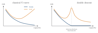
Message: interesting, unresolved, and not our topic. Our practical answer to “will it generalize?” is experimental hygiene — proper splits, honest evaluation — built in U0.L2.

Why this matters later: generative models are trained by the same optimizers on the same kind of surfaces. Nothing new will be needed.

04MLPs and universal approximation

The multilayer perceptron

An MLP with \(L\) layers is the composition \[ x^{0} = x, \qquad x^{k} = \sigma\big(W_k\, x^{k-1} + b_k\big) \quad (k = 1, \dots, L-1), \qquad f_\theta(x) = W_L\, x^{L-1} + b_L, \] with \(\theta = \{W_k, b_k\}_{k=1}^{L}\) and \(\sigma\) an elementwise activation.

Activations: ReLU and its family for intuition; SiLU / GELU are what we will actually use in U-Nets and DiT (U0.T4 onward).

The shape of the thing

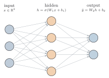
• Width: each layer mixes and rectifies features.
• Depth: \(f_\theta = f_L \circ f_{L-1} \circ \cdots \circ f_1\) — a composition. Hold this thought; it is the whole of Block E.

Universal approximation — statement only

Let \(\sigma : \mathbb{R} \to \mathbb{R}\) be continuous and non-polynomial, and \(K \subset \mathbb{R}^d\) compact. Then the one-hidden-layer networks \[ \Big\{\, x \mapsto \textstyle\sum_{j=1}^{N} a_j\, \sigma\big(w_j^{\top} x + b_j\big) \;:\; N \in \mathbb{N},\; a_j, b_j \in \mathbb{R},\; w_j \in \mathbb{R}^d \,\Big\} \] are dense in \(C(K)\) with the sup norm: every continuous function on \(K\) is uniformly approximable.

Two caveats, same slide: (i) this says nothing about learnability — existence of a good network, not of an algorithm that finds it; (ii) width/depth tradeoffs are not quantified here (\(N\) may be astronomically large).

Why later — and the segue

In U1.T2 we meet universality questions again for invertible models — where the answer is subtler because invertibility is a real constraint. Keep today’s fine print in mind.

Depth as composition: \[ f_\theta \;=\; f_L \circ f_{L-1} \circ \cdots \circ f_1 . \]

Training minimizes \(\widehat{R}_n(\theta)\) by gradient descent — so we need derivatives of long compositions, cheaply. That is a question about computational graphs.

05Backprop as reverse-mode autodiff

Computational graphs

A numerical program is a computational graph: nodes are primitive operations (matmul, add, \(\sigma\), …), edges carry data. Evaluating \(\mathcal{L}(\theta)\) runs the graph forward — and caches the intermediates \(x^{1}, x^{2}, \dots\)

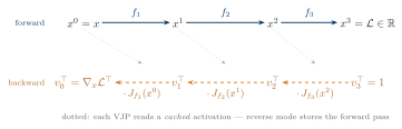
A chain graph: forward pass above, cotangent pass below. Today’s mental model.

Differentiation will be another pass over the same graph; the only questions are direction and cost.

The primitive: vector–Jacobian products

For a primitive \(f : \mathbb{R}^n \to \mathbb{R}^m\), differentiable at \(x\), and an upstream cotangent (row vector) \(v^{\top} \in \mathbb{R}^{1 \times m}\), the vector–Jacobian product is \[ \mathrm{VJP}_f(v; x) \;=\; v^{\top} J_f(x) \;\in\; \mathbb{R}^{1 \times n}, \qquad J_f(x) = \frac{\partial f}{\partial x} \in \mathbb{R}^{m \times n}. \]

Insist on the row-vector view — not “gradients of everything.” Each primitive ships a backward op \(v \mapsto v^{\top} J_f(x)\) computable at roughly the cost of one forward evaluation, without materializing \(J_f(x)\). This is what makes reverse mode \(O(1\ \text{forward-cost})\) per scalar output.

Live proof: VJP composition

Let \(h = g \circ f\) with \(f\) differentiable at \(x\) and \(g\) differentiable at \(f(x)\). By the chain rule \(J_h(x) = J_g(f(x))\, J_f(x)\), and for any cotangent \(v\): \[ v^{\top} J_h(x) \;=\; \big(v^{\top} J_g(f(x))\big)\, J_f(x), \qquad\text{i.e.}\qquad \mathrm{VJP}_h(v; x) = \mathrm{VJP}_f\big(\mathrm{VJP}_g(v;\, f(x));\; x\big). \]

Proof (two-layer case). Matrix multiplication is associative: \(v^{\top}(J_g J_f) = (v^{\top} J_g) J_f\). That is the whole proof — the content is in the reading: the left side forms a \(p \times n\) Jacobian product; the right side is two matrix–vector products. \(\square\)

Board 2: two-node graph, VJP composition proof. Do not erase before the cost-table discussion — point at it.

From two layers to L: right-to-left accumulation

For \(h = f_L \circ \cdots \circ f_1\) with intermediates \(x^{k} = f_k(x^{k-1})\), iterate the Proposition: \[ v_L^{\top} = v^{\top}, \qquad v_{k-1}^{\top} \;=\; v_k^{\top}\, J_{f_k}\big(x^{k-1}\big), \qquad v_0^{\top} \;=\; v^{\top} J_h(x^{0}). \]

Reverse-mode autodiff = right-to-left accumulation of VJPs. The induction on \(L\) is one line (in the notes, boxed — we will cite that box again in U2.T1).

Backprop is exactly this, with \(v^{\top} = 1\) on the scalar loss \(\mathcal{L}\) — the cotangent sweeps the graph backwards, \(k = L, \dots, 1\).

Cost accounting: forward vs. reverse

For \(h : \mathbb{R}^n \to \mathbb{R}^m\) built from primitives (one pass \(\approx\) constant \(\times\) forward cost):

	one pass computes	full Jacobian needs	scalar loss (\(m = 1\))
Forward mode (JVP)	\(J_h(x)\, u\) — one input direction	\(n\) passes	\(n\) passes
Reverse mode (VJP)	\(v^{\top} J_h(x)\) — one output direction	\(m\) passes	1 pass

Training loss: \(n = \dim \theta\) (millions), \(m = 1\). Reverse mode computes \(\nabla_\theta \mathcal{L}\) at the cost of a constant number of forward passes — this asymmetry is why deep learning is possible at scale.

The coverage race, animated

The price: memory

Each VJP \(v_k^{\top} J_{f_k}(x^{k-1})\) needs the activation \(x^{k-1}\) — reverse mode must store the forward pass (the dotted arrows in the graph figure). Memory grows with depth. Flag it now; it is not a footnote.

Memory of activations is precisely what the adjoint method (U2.T1) trades against recomputation-by-integration: instead of storing states, it recovers them by solving the dynamics backwards.

The reverse sweep, animated

06The bridge, and what’s next

Backprop \(\to\) adjoint

Backprop (today)

• discrete composition \(\;x_{k+1} = f_k(x_k)\)
• cotangent runs backwards \(\;k = L, \dots, 1\)
• stores activations

Adjoint (U2, week ~8)

• continuous composition \(\;\mathrm{d}x/\mathrm{d}t = u_t(x)\)
• costate runs backwards \(\;t = 1 \to 0\)
• recomputes states by solving the ODE in reverse

“Backprop is the discrete ancestor of the adjoint method.”

Close: PS0 and the next session

• PS0 preview, one line: a VAE with your own U-Net and your own evaluation harness — every part gets built in this unit.
• Next session (U0.L1): PyTorch from zero. Bring laptops; environment instructions are posted today.

See you next session.