UP.A — Probability for Generative Models
Session UP.A · async primer · date: see calendar-map
How to read this page. This is the async primer of the course, and it is a document rather than a lecture. There are no slides, and nothing here was said out loud in a room you might have missed. It is written to be read alone, at your own pace, before the first live session.
It is also self-contained. Every formula this course later uses is derived here, on this page, from the definitions given here. No proof below sends you to a textbook to fill a gap. Two books are named at the end of each section as a slower treatment of the same material — (Bishop and Bishop 2024) chapters 2–3, and (Murphy 2023) chapters 2 and 5 — and they are optional, every one of them. Each section names the chapter that matches it.
The primer serves two populations at once. If you come from computer science, plan to grind: read with a pen, and do the exercises. If you come from mathematics, plan to skim: every section opens with a short self-test, and if you answer it comfortably you may go to the next section. The self-test answers are in a footnote, so you can check yourself without reading ahead.
Every section ends with exercises tagged [PS1.1.x]. Those nine exercises are problem set PS1.1, and PS1.1 is part of PS1, which carries about 12% of the course grade. They are not optional practice. Answers are not printed here, because you will hand them in.
One more thing to know before you start. Each section ends with a box titled “Where this reappears”, naming the sessions that consume it by session ID. Nothing on this page is here for general culture. Every item was put here because a specific later session needs it, and the box tells you which one.
The notation of this course is fixed, and this page is your first exposure to it. Section 5 drills it, and Appendix A reproduces the full symbol table.
§1 — Densities and conditioning
- A joint density \(p(x, y)\) is given. Write the marginal \(p(y)\) and the conditional \(p(x \mid y)\) in terms of it.
- \(X\) and \(Y\) are each fair coin flips, and \(Z = X \oplus Y\) is their exclusive or. Are \(X\) and \(Y\) independent? Are they independent given \(Z\)?
- You draw \(Y \sim \mathrm{Unif}\{1, 2\}\), then \(X \sim \mathcal{N}(Y, 1)\). What is \(\mathbb{E}[X]\)?
Answers in the footnote.1
Joint, marginal, conditional
Everything in this course is built out of three operations on one object. The object is a joint density, and the operations are marginalizing, conditioning, and taking expectations.
A function \(p \colon \mathbb{R}^{d_x} \times \mathbb{R}^{d_y} \to [0, \infty)\) is a joint density for the pair \((X, Y)\) if \[ \mathbb{P}\big[(X, Y) \in A\big] \;=\; \int_A p(x, y)\,\mathrm{d}x\,\mathrm{d}y \] for every (measurable) set \(A\), and \(\int p(x,y)\,\mathrm{d}x\,\mathrm{d}y = 1\).
A density is not a probability. It is a probability per unit volume, and it may exceed \(1\). What is bounded by \(1\) is its integral over a region.
Marginalizing removes a variable by integrating it away: \[ p(y) \;=\; \int p(x, y)\,\mathrm{d}x . \tag{1}\]
Read Equation 1 as summing out \(x\): you no longer care which value \(X\) took, so you add up the mass over all of them. The result is a density in \(y\) alone, and the same symbol \(p\) is used for it. The argument list tells you which density is meant. This overloading is universal in the field, and this course keeps it.
Conditioning fixes a variable and renormalizes what is left:
\[ p(x \mid y) \;=\; \frac{p(x, y)}{p(y)} , \qquad \text{wherever } p(y) > 0 . \tag{2}\]
Figure 1 is the picture behind Equation 2, and it is worth more than the formula. Conditioning is two steps, and they are different steps. First you cut: fix \(y = y_0\) and keep only the values of the joint along that line. Second you renormalize: divide by the mass you just cut, so the result is again a density.
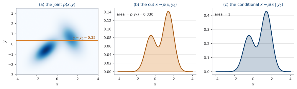
The three panels of Figure 1 show the results of those two steps. The animation below shows the steps themselves, which is the part a static figure has to leave to the reader. The cutting plane sweeps down through the joint and stops at \(y_0 = 0.35\); the cut is drawn in accent colour, because it is not yet a density; its area is measured on screen and comes to \(p(y_0) = 0.330\), and the caption says plainly that this is not \(1\). Only then does the division happen, as a vertical inflation by the factor \(1/p(y_0) = 3.03\), with the undivided cut left behind in gray so the two can be compared:
Watch the shape while it inflates. It does not change — only the height does. That is the single most useful thing to take from the scene, because the common misreading of Equation 2 is that the conditional is “the joint, restricted”, which is the cut and not the division. The cut alone is a perfectly good function and a perfectly bad density.
Three consequences of Equation 2 deserve to be stated, because each one is used later without comment.
The chain rule. Multiply Equation 2 out and you get \(p(x, y) = p(x \mid y)\, p(y)\). This is how a joint gets built rather than analyzed: choose a marginal, then choose a conditional. Every generative model in this course is built that way.
Bayes’ rule. Apply the chain rule both ways and divide:
\[ p(y \mid x) \;=\; \frac{p(x \mid y)\, p(y)}{p(x)} , \qquad p(x) \;=\; \int p(x \mid y)\, p(y) \,\mathrm{d}y . \tag{3}\]
Conditioning on the wrong thing gives the wrong answer. \(p(x \mid y)\) and \(p(y \mid x)\) are different functions of different arguments, and the whole content of Equation 3 is the exchange rate between them.
Let \(Y \in \{0, 1\}\) be a class label with \(\mathbb{P}[Y = 1] = \pi\), and let the feature \(X \in \mathbb{R}\) satisfy \(X \mid Y = k \sim \mathcal{N}(\mu_k, \sigma^2)\). The two variables are of different types, and Equation 3 handles both directions anyway.
Forward, the density of \(X\) is a mixture: \[ p(x) \;=\; (1 - \pi)\, \mathcal{N}(x; \mu_0, \sigma^2) \;+\; \pi\, \mathcal{N}(x; \mu_1, \sigma^2) . \]
Backward, the posterior on the label is a number in \([0,1]\): \[ \mathbb{P}[Y = 1 \mid X = x] \;=\; \frac{\pi\, \mathcal{N}(x; \mu_1, \sigma^2)} {(1-\pi)\, \mathcal{N}(x; \mu_0, \sigma^2) + \pi\, \mathcal{N}(x; \mu_1, \sigma^2)} . \]
Put \(\mu_0 = -1\), \(\mu_1 = +1\), \(\sigma = 1\), \(\pi = 1/2\) and simplify: the Gaussian normalizers cancel, and what survives is \(\mathbb{P}[Y=1 \mid X=x] = \sigma_{\mathrm{logistic}}(2x)\), the logistic function of \(2x\). A logistic regression is what Bayes’ rule becomes under equal-covariance Gaussian classes. This is worth remembering, and it is worth remembering that it is a consequence, not a definition.
Independence, and why the conditional version is different
\(X\) and \(Y\) are independent, written \(X \perp Y\), when \(p(x, y) = p(x)\,p(y)\) for all \(x, y\). Equivalently, \(p(x \mid y) = p(x)\): learning \(Y\) tells you nothing about \(X\).
They are conditionally independent given \(Z\), written \(X \perp Y \mid Z\), when \(p(x, y \mid z) = p(x \mid z)\, p(y \mid z)\) for all \(z\) with \(p(z) > 0\). Learning \(Y\) tells you nothing about \(X\) that you did not already know from \(Z\).
Neither statement implies the other. Both failures happen, and both are common.
One number is used below to summarize how two coordinates move together, and it is worth defining before the picture. The correlation of \(X\) and \(Y\) is \[ \rho \;=\; \frac{\operatorname{Cov}(X, Y)}{\sigma_X \sigma_Y}, \qquad \operatorname{Cov}(X, Y) = \mathbb{E}_{(x,y) \sim p}\big[(x - \mu_X)(y - \mu_Y)\big] . \tag{4}\] It lies in \([-1, 1]\). It is zero when the two carry no linear relation, and \(\pm 1\) when one is an affine function of the other. The sample correlation is the same formula with the two expectations replaced by averages over a finite sample, and it is what Figure 2 reports.
Zero correlation is weaker than independence, and the gap matters: independent variables always have zero correlation, and variables with zero correlation may still be strongly dependent, through a relation that is not linear.
Figure 2 shows the direction that matters most for us. A hidden variable \(Z\) chooses one of two clusters. Given \(Z\), the two coordinates are drawn independently, so each cluster is round: within a cluster, knowing \(x\) tells you nothing about \(y\). Hide \(Z\), and the two clusters lie along a line, so the sample correlation is \(0.85\). The dependence between \(X\) and \(Y\) was manufactured entirely by the variable you cannot see.
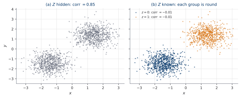
This picture is not decoration. The whole of this course builds complicated distributions in exactly this way: pick a latent variable, make everything simple given that variable, and let the marginal be complicated as a consequence. Figure 2 is the smallest possible instance of that idea.
Expectations, and the subscripts this course requires
For a function \(g\) and a random variable \(X\) with density \(p\), \[ \mathbb{E}_{x \sim p}\big[g(x)\big] \;=\; \int g(x)\, p(x)\, \mathrm{d}x , \] whenever the integral converges absolutely.
Expectation is linear: for constants \(a, b\) and functions \(g, h\), \(\mathbb{E}_{x\sim p}[a\,g(x) + b\,h(x)] = a\,\mathbb{E}_{x\sim p}[g(x)] + b\,\mathbb{E}_{x\sim p}[h(x)]\). Linearity needs no independence, no assumption at all beyond convergence. It is the single most used fact in the course.
Now the notation rule, and it is a rule rather than a preference.
Whenever more than one distribution is in play, every \(\mathbb{E}\) carries an explicit subscript naming the variable and the distribution it is drawn from. Write \(\mathbb{E}_{x \sim p}\), never a bare \(\mathbb{E}\).
The reason is not tidiness. Consider the expression \[ \mathbb{E}\big[\,\|f_\theta(y) - x\|^2\,\big] . \] There are three symbols in it, and the bare \(\mathbb{E}\) does not say which of them are averaged over. Is \(y\) drawn and \(x\) held fixed? Are both drawn, and jointly or independently? Is \(\theta\) random? Every one of those readings is a different quantity, and at least two of them appear in real papers. Written in the standard of this course, the ambiguity cannot survive: \[ \mathbb{E}_{(x, y) \sim p}\big[\,\|f_\theta(y) - x\|^2\,\big] , \] which says: the pair is drawn jointly from \(p\), and \(\theta\) is a parameter, not a random variable. Section 5 drills this until it is automatic.
The law of total expectation, informally. Suppose you draw \(Y\), then draw \(X\) given \(Y\). You can compute \(\mathbb{E}[X]\) in one pass, or in two: average \(X\) within each value of \(Y\) first, then average those averages over \(Y\).
\[ \mathbb{E}_{x \sim p}\big[X\big] \;=\; \mathbb{E}_{y \sim p}\Big[\, \mathbb{E}_{x \sim p(\cdot \mid y)}\big[X\big] \,\Big] . \tag{5}\]
Equation 5 is stated here for intuition, and used here only on examples where you could check it by hand. The formal statement, the hypotheses under which it holds, and its proof are the opening act of UP.T1. Do not cite this equation as proved. Build the intuition now; the theorem comes later.
Draw \(Y\) uniformly from \(\{1, 2, 3\}\), then draw \(X \mid Y = k \sim \mathcal{N}(k^2, 1)\).
Directly. The density of \(X\) is the mixture \(\tfrac13 \sum_{k=1}^{3} \mathcal{N}(x; k^2, 1)\), and the mean of a mixture is the mixture of the means, so \(\mathbb{E}[X] = \tfrac13 (1 + 4 + 9) = 14/3\).
By Equation 5. The inner expectation is \(\mathbb{E}_{x \sim p(\cdot \mid y)}[X] = y^2\), a function of \(y\). Averaging that function over \(Y\) gives \(\tfrac13(1^2 + 2^2 + 3^2) = 14/3\).
The two routes agree, which is the point. The second route is the one that scales, because the inner expectation is often available in closed form when the outer one is not. Notice also what the inner expectation is: not a number, but a function of the conditioning variable. That observation is the seed of UP.T1.
- UP.T1 proves Equation 5 properly, and then proves the projection Lemma — the central technical device of this course — out of it.
- U3.T1 marginalizes a family of conditional densities exactly as Equation 1 does here, over a variable that will be a data point.
- The mandatory subscripts of Section 1.3 appear in every loss in every remaining session, without exception.
Exercises for §1
[PS1.1.1] Let \(p(x, y) = c\) on the region \(\{(x,y) : 0 \le y \le 1,\ 0 \le x \le 1 + y\}\) and \(p(x,y) = 0\) elsewhere.
- Find \(c\). (b) Compute the marginal \(p(y)\) and the marginal \(p(x)\); note that they are not of the same form. (c) Compute the conditional \(p(x \mid y)\) and state, in one sentence, how it depends on \(y\). (d) Compute \(p(y \mid x)\) for \(x = 1/2\) and for \(x = 3/2\), and explain why the two answers have different supports.
[PS1.1.2] Draw \(Y \sim \mathrm{Exp}(1)\), then \(X \mid Y = y \sim \mathcal{N}(y, y^2)\).
- Compute \(\mathbb{E}[X]\) directly, by first writing the density of \(X\) as an integral and exchanging the order of integration. (b) Compute \(\mathbb{E}[X]\) by Equation 5. (c) Compute \(\mathbb{E}[X^2]\) by Equation 5, and hence \(\operatorname{Var}(X)\). (d) State which of the two routes you would want if the conditional law were \(\mathcal{N}(y, y^2)\) but \(Y\) had a density you could only sample from, not integrate against.
Slower treatment of §1, optional: (Bishop and Bishop 2024) ch. 2, (Murphy 2023) ch. 2.
§2 — Gaussian algebra
- \(x \sim \mathcal{N}(\mu, \Sigma)\) and \(A\) is a matrix. What is the law of \(Ax + b\)?
- \((x_a, x_b)\) is jointly Gaussian. Is \(x_a \mid x_b\) Gaussian? Is its covariance a function of \(x_b\)?
- Write \(x^\top A x - 2 b^\top x\) as a single squared term plus a constant.
Answers in the footnote.2
This section is the workhorse of the course. Almost every closed-form computation in the remaining fourteen weeks is one of the five results below, applied to a specific pair of matrices. The boxed formulas of this section ship separately as the two-page gaussian-algebra-toolkit sheet (see the toolkit page); later sessions consume it by that name.
2.1 The Gaussian, and the first pushforward
For \(\mu \in \mathbb{R}^d\) and a symmetric positive definite \(\Sigma \in \mathbb{R}^{d \times d}\), \[ \mathcal{N}(x; \mu, \Sigma) \;=\; \frac{1}{(2\pi)^{d/2} \,(\det \Sigma)^{1/2}} \exp\!\Big( -\tfrac12 (x - \mu)^\top \Sigma^{-1} (x - \mu) \Big) . \tag{6}\] The standard Gaussian is \(\mathcal{N}(0, I_d)\). In this course it is the source distribution, written \(p_0\), and its samples are written \(x_0\).
The exponent of Equation 6 is a quadratic form in \(x\), and the prefactor is whatever makes the integral equal \(1\). That is the entire structure. Every manipulation in this section is a manipulation of the quadratic form, with the prefactor recovered at the end by inspection.
Here is the first, and the one that names the pattern.
Let \(z \sim \mathcal{N}(0, I_d)\) and let \(\Sigma^{1/2}\) be any matrix with \(\Sigma^{1/2} (\Sigma^{1/2})^\top = \Sigma\). Then \[ x \;=\; \mu + \Sigma^{1/2} z \;\sim\; \mathcal{N}(\mu, \Sigma) . \tag{7}\]
Read Equation 7 as a recipe, not as an identity. It says: to obtain a sample from a complicated Gaussian, draw from the simple one and push the sample through a deterministic map. The distribution on the left is the image of the distribution on the right under that map, and the technical name for such an image is a pushforward. UP.T1 defines pushforwards properly and proves what this section only exhibits. Keep the shape of Equation 7 in mind: fixed simple source, deterministic map, the interesting distribution as the image. It recurs.
2.2 Linear transforms
\[ x \sim \mathcal{N}(\mu, \Sigma) \quad\Longrightarrow\quad A x + b \;\sim\; \mathcal{N}\!\big(A\mu + b,\; A \Sigma A^\top\big) . \tag{8}\]
Two things have to be shown, and they are shown differently.
The moments. By linearity of expectation, \(\mathbb{E}_{x \sim \mathcal{N}(\mu, \Sigma)}[Ax + b] = A\mu + b\). For the covariance, write \(y = Ax + b\) and \(\bar y = A\mu + b\), so that \(y - \bar y = A(x - \mu)\) and \[ \begin{aligned} \operatorname{Cov}(y) &= \mathbb{E}_{x \sim \mathcal{N}(\mu, \Sigma)}\big[A(x-\mu)(x-\mu)^\top A^\top\big] \\ &= A\,\mathbb{E}_{x \sim \mathcal{N}(\mu, \Sigma)}\big[(x-\mu)(x-\mu)^\top\big]\,A^\top = A \Sigma A^\top . \end{aligned} \] The matrix \(A\) comes out of the expectation because it is constant, and what remains inside is the definition of \(\Sigma\).
The family. Moments alone are not enough: a non-Gaussian variable can share the first two moments of a Gaussian. What closes the argument is that the Gaussian family is closed under affine maps, and Equation 7 is the reason. If \(x = \mu + \Sigma^{1/2} z\) with \(z\) standard, then \[ Ax + b \;=\; (A\mu + b) \;+\; (A\Sigma^{1/2}) z , \] which is again an affine map of a standard Gaussian, hence again Gaussian by Equation 7, with covariance \((A\Sigma^{1/2})(A\Sigma^{1/2})^\top = A \Sigma A^\top\). The two computations together give Equation 8.
This course does not use characteristic functions anywhere, and it does not need them. Equation 7 plus moment matching is the whole toolkit.
One immediate corollary, which will do the work in Section 2.5: taking \(A = \begin{bmatrix} 0 & I \end{bmatrix}\) selects a sub-vector. A marginal of a jointly Gaussian vector is Gaussian, and you read its mean and covariance directly off the corresponding blocks.
2.3 Sums of independent Gaussians
\[ \begin{aligned} x \sim \mathcal{N}(\mu_x, \Sigma_x),\quad y \sim \mathcal{N}(\mu_y, \Sigma_y),\quad x \perp y \\ \Longrightarrow\quad x + y \sim \mathcal{N}(\mu_x + \mu_y,\; \Sigma_x + \Sigma_y) . \end{aligned} \tag{9}\]
This follows from Equation 8 applied to the stacked vector \(\begin{bmatrix} x \\ y\end{bmatrix}\), which is Gaussian with block-diagonal covariance precisely because \(x\) and \(y\) are independent, under the map \(A = \begin{bmatrix} I & I \end{bmatrix}\). Independence is what makes the covariance block-diagonal, and hence what makes the variances add. Without it, Equation 9 is false, and the cross-covariance terms survive.
Now the special case that the whole second half of the course is built on.
Let \(x_0 \sim \mathcal{N}(0, I_d)\), let \(x_1 \in \mathbb{R}^d\) be fixed, and let \(\alpha, \sigma \in \mathbb{R}\) with \(\sigma > 0\). Then \[ \alpha x_1 + \sigma x_0 \;\sim\; \mathcal{N}\big(\alpha x_1,\; \sigma^2 I_d\big) . \tag{10}\] If instead \(x_1\) is itself random, drawn from \(q\) and independent of \(x_0\), then 1 is the law conditional on \(x_1\), and the unconditional law of \(\alpha x_1 + \sigma x_0\) is a mixture of Gaussians, one per value of \(x_1\).
The proof is one line of Equation 8 with \(A = \sigma I_d\) and \(b = \alpha x_1\). The content is entirely in the conditional qualifier, and in Section 1.2’s picture: simple given the latent, complicated once the latent is hidden.
1 is the entire mechanism of the Gaussian probability paths of U3.T1 item 4. There, the two constants become functions of time, \(\alpha_t\) and \(\sigma_t\), and the family of laws they generate as \(t\) runs from \(0\) to \(1\) is the object the course spends four weeks on. Nothing else changes. The algebra you are reading now is the algebra you will use then.
2.4 Completing the square
Every remaining derivation in this section is one application of the following identity. It is worth learning by heart, because it is the only trick.
Let \(A\) be symmetric and invertible, and let \(b\) be a vector. Then \[ x^\top A x \;-\; 2\, b^\top x \;=\; (x - A^{-1} b)^\top A\, (x - A^{-1} b) \;-\; b^\top A^{-1} b . \tag{11}\]
Proof. Expand the first term on the right: \[ (x - A^{-1}b)^\top A (x - A^{-1}b) = x^\top A x - x^\top A A^{-1} b - b^\top A^{-1} A x + b^\top A^{-1} A A^{-1} b . \] The two middle terms are each the scalar \(b^\top x\), because \(A\) is symmetric and so is \(A^{-1}\); the last term is \(b^\top A^{-1} b\). Subtracting \(b^\top A^{-1} b\) from both sides gives Equation 11. \(\square\)
The way to use Equation 11 is always the same, and it is worth spelling out once. You have an exponent that is quadratic in some variable \(x\). You collect it into the shape \(-\tfrac12 (x^\top A x - 2 b^\top x) + \text{const}\). You apply Equation 11. What you read off is that the density is Gaussian in \(x\) with covariance \(A^{-1}\) and mean \(A^{-1} b\) — and the leftover constant \(-\tfrac12 b^\top A^{-1} b\) does not depend on \(x\), so it is absorbed into the normalizer and never has to be computed.
That last point is what makes the method cheap. You never track the prefactor. You identify the quadratic form, and the prefactor is whatever normalizes it.
2.5 Conditionals and marginals of a joint Gaussian
This is the centerpiece of the primer. Let \(z = \begin{bmatrix} x_a \\ x_b \end{bmatrix}\) be jointly Gaussian, with the blocks \[ \mu = \begin{bmatrix} \mu_a \\ \mu_b \end{bmatrix}, \qquad \Sigma = \begin{bmatrix} \Sigma_{aa} & \Sigma_{ab} \\ \Sigma_{ba} & \Sigma_{bb} \end{bmatrix}, \qquad \Sigma_{ba} = \Sigma_{ab}^\top . \]
The marginals are free. By the corollary of Section 2.2, \(x_a \sim \mathcal{N}(\mu_a, \Sigma_{aa})\) and \(x_b \sim \mathcal{N}(\mu_b, \Sigma_{bb})\). You read them off the blocks, and there is nothing to compute.
The conditional takes one application of Equation 11. Write \(\Lambda = \Sigma^{-1}\) in blocks, \(\Lambda_{aa}, \Lambda_{ab}, \Lambda_{bb}\). The exponent of the joint density is \(-\tfrac12 (z - \mu)^\top \Lambda (z - \mu)\), and expanding the blocks with \(u = x_a - \mu_a\) and \(w = x_b - \mu_b\) gives \[ -\tfrac12\Big( u^\top \Lambda_{aa} u \;+\; 2\, u^\top \Lambda_{ab} w \;+\; w^\top \Lambda_{bb} w \Big). \] Now fix \(x_b\), so that \(w\) is a constant. The last term is constant, and drops into the normalizer. What remains is quadratic in \(u\), in exactly the shape Equation 11 wants, with \(A = \Lambda_{aa}\) and \(b = -\Lambda_{ab} w\). Reading off the mean and covariance: \[ \begin{aligned} x_a \mid x_b \;\sim\; \mathcal{N}\big( m,\; C \big), \qquad m &= \mu_a - \Lambda_{aa}^{-1} \Lambda_{ab}(x_b - \mu_b), \\ C &= \Lambda_{aa}^{-1} . \end{aligned} \tag{12}\]
Equation 12 is already the answer, but it is written in the blocks of the inverse covariance, and you are usually handed \(\Sigma\). The translation is one identity.
Write \(S = \Sigma_{aa} - \Sigma_{ab} \Sigma_{bb}^{-1} \Sigma_{ba}\), the Schur complement of \(\Sigma_{bb}\). If \(\Sigma\) and \(\Sigma_{bb}\) are invertible, so is \(S\), and \[ \Lambda_{aa} \;=\; S^{-1} , \qquad \Lambda_{ab} \;=\; -\,S^{-1} \Sigma_{ab} \Sigma_{bb}^{-1} . \tag{13}\]
Proof. It is enough to exhibit a matrix and check that it is the inverse. Take \(\Lambda_{aa} = S^{-1}\), \(\Lambda_{ab} = -S^{-1}\Sigma_{ab}\Sigma_{bb}^{-1}\) and \(\Lambda_{bb} = \Sigma_{bb}^{-1} + \Sigma_{bb}^{-1}\Sigma_{ba} S^{-1}\Sigma_{ab}\Sigma_{bb}^{-1}\). Multiplying out \(\Sigma \Lambda\) block by block, the top-left block is \(\Sigma_{aa} S^{-1} - \Sigma_{ab}\Sigma_{bb}^{-1}\Sigma_{ba}S^{-1} = S S^{-1} = I\), and the top-right block is \(-\Sigma_{aa}S^{-1}\Sigma_{ab}\Sigma_{bb}^{-1} + \Sigma_{ab}\Sigma_{bb}^{-1} + \Sigma_{ab}\Sigma_{bb}^{-1}\Sigma_{ba}S^{-1}\Sigma_{ab}\Sigma_{bb}^{-1} = (-S S^{-1} + I)\,\Sigma_{ab}\Sigma_{bb}^{-1} = 0\). The two lower blocks are the same computation transposed. \(\square\)
Substituting Equation 13 into Equation 12 gives the formula this course uses. Note that \(\Lambda_{aa}^{-1}\Lambda_{ab} = -\Sigma_{ab}\Sigma_{bb}^{-1}\), so the two minus signs cancel.
\[ \boxed{\; x_a \mid x_b \;\sim\; \mathcal{N}\Big(\; \mu_a + \Sigma_{ab}\Sigma_{bb}^{-1}(x_b - \mu_b), \;\; \Sigma_{aa} - \Sigma_{ab}\Sigma_{bb}^{-1}\Sigma_{ba} \;\Big) \; } \tag{14}\]
Three observations, each of which is used later.
The conditional mean is affine in \(x_b\). It is the marginal mean, corrected by a linear function of how far \(x_b\) landed from its mean. The correction matrix \(\Sigma_{ab}\Sigma_{bb}^{-1}\) is a regression coefficient, and if \(\Sigma_{ab} = 0\) it vanishes — uncorrelated jointly Gaussian variables are independent, which is a Gaussian privilege and false in general.
The conditional covariance does not depend on \(x_b\) at all. Observing \(x_b\) reduces your uncertainty about \(x_a\) by the same amount no matter what value you observe. This is peculiar to the Gaussian family, and it is the single property that makes everything downstream tractable.
Conditioning never increases the covariance. The subtracted term \(\Sigma_{ab}\Sigma_{bb}^{-1}\Sigma_{ba}\) is positive semidefinite, so \(S \preceq \Sigma_{aa}\). Information cannot hurt.
The scalar corollary
You will use the one-dimensional case constantly, so it is written out separately. Let \((X, Y)\) be jointly Gaussian with means \(\mu_X, \mu_Y\), variances \(\sigma_X^2, \sigma_Y^2\) and covariance \(\sigma_{XY}\).
\[ X \mid Y = y \;\sim\; \mathcal{N}\Big(\; \mu_X + \frac{\sigma_{XY}}{\sigma_Y^2}\,(y - \mu_Y), \;\; \sigma_X^2 - \frac{\sigma_{XY}^2}{\sigma_Y^2} \;\Big) . \tag{15}\]
Writing \(\rho = \sigma_{XY}/(\sigma_X \sigma_Y)\) for the correlation, the conditional variance is \(\sigma_X^2 (1 - \rho^2)\): the fraction of the variance of \(X\) that observing \(Y\) does not explain.
2.6 A worked example, to be remembered
Let \(X \sim \mathcal{N}(\mu_0, \sigma_0^2)\), and suppose you do not observe \(X\) itself but a corrupted version of it, \[ Y \;=\; X + \sigma \varepsilon , \qquad \varepsilon \sim \mathcal{N}(0, 1), \qquad \varepsilon \perp X . \] What is the best guess of \(X\) given \(Y = y\)?
Step 1 — the pair is jointly Gaussian. The vector \((X, Y)\) is an affine map of the independent Gaussian pair \((X, \varepsilon)\), namely \(\begin{bmatrix} X \\ Y \end{bmatrix} = \begin{bmatrix} 1 & 0 \\ 1 & \sigma \end{bmatrix} \begin{bmatrix} X \\ \varepsilon \end{bmatrix}\), so Equation 8 applies and the pair is Gaussian.
Step 2 — read off the moments. Both means are \(\mu_0\). The variances are \(\sigma_X^2 = \sigma_0^2\) and, by Equation 9, \(\sigma_Y^2 = \sigma_0^2 + \sigma^2\). The covariance is \[ \sigma_{XY} = \mathbb{E}\big[(X - \mu_0)(X - \mu_0 + \sigma\varepsilon)\big] = \sigma_0^2 , \] since the cross term vanishes by independence and \(\mathbb{E}[\varepsilon] = 0\).
Step 3 — apply Equation 15. With \(\sigma_{XY} = \sigma_0^2\) and \(\sigma_Y^2 = \sigma_0^2 + \sigma^2\): \[ \begin{aligned} \mathbb{E}\big[X \mid Y = y\big] &\;=\; \frac{\sigma_0^2}{\sigma_0^2 + \sigma^2}\, y \;+\; \frac{\sigma^2}{\sigma_0^2 + \sigma^2}\, \mu_0 , \\[2pt] \operatorname{Var}\big(X \mid Y = y\big) &\;=\; \frac{\sigma_0^2 \sigma^2}{\sigma_0^2 + \sigma^2} . \end{aligned} \tag{16}\]
Read the answer. Equation 16 is a weighted average of the observation \(y\) and the prior mean \(\mu_0\), and the weights are the two variances, swapped. Clean observation (\(\sigma \to 0\)): the weight goes to \(y\), and you trust what you saw. Hopeless observation (\(\sigma \to \infty\)): the weight goes to \(\mu_0\), and you fall back on what you believed. The conditional variance is smaller than both \(\sigma_0^2\) and \(\sigma^2\), which is the statement that two noisy sources beat either one alone.
It looks like nothing more than an exercise in Equation 15, and on this page that is exactly what it is. It has a secret identity. The reveal is scheduled, and it is one of the better moments of the course. Copy the formula somewhere you will find it again.
- U3.T1 item 4 builds its conditional families out of 1, with \(\alpha_t\) and \(\sigma_t\) in place of the two constants.
- Detour D1 studies which choices of those two functions of time recover which classical constructions.
- Detour D2 rests on Equation 16, in the form it takes when the reveal happens.
- UP.T1 reuses the example of Section 2.6 for problem set PS1.2.
- The boxed formulas of this section are the
gaussian-algebra-toolkitsheet, consumed by name in the U3 sessions.
Exercises for §2
[PS1.1.3] Let \((X_1, X_2)\) be jointly Gaussian with mean \((1, -2)\) and covariance \(\Sigma = \begin{bmatrix} 4 & 2 \\ 2 & 3 \end{bmatrix}\).
- Write \(X_1 \mid X_2 = x_2\) explicitly, using Equation 15. (b) Compute the correlation \(\rho\) and verify that the conditional variance equals \(\sigma_{X_1}^2 (1 - \rho^2)\). (c) Invert \(\Sigma\) by hand and confirm Equation 13 on this example, that is, confirm \(\Lambda_{11} = S^{-1}\) with \(S = \Sigma_{11} - \Sigma_{12}\Sigma_{22}^{-1}\Sigma_{21}\). (d) By how much does observing \(X_2\) reduce the variance of \(X_1\), as a percentage?
[PS1.1.4] Let \(x_0 \sim \mathcal{N}(0, I_d)\) and let \(x_1 \sim q\) be independent of \(x_0\), where \(q\) is any distribution on \(\mathbb{R}^d\) with mean \(m\) and covariance \(C\) (not Gaussian, and not otherwise specified). Fix constants \(\alpha, \sigma\) and set \(x = \alpha x_1 + \sigma x_0\).
- Show that \(x \mid x_1 \sim \mathcal{N}(\alpha x_1, \sigma^2 I_d)\), which is
- Compute \(\mathbb{E}[x]\) using Equation 5. (c) Compute \(\operatorname{Cov}(x)\) using the law of total variance, \(\operatorname{Cov}(x) = \mathbb{E}[\operatorname{Cov}(x \mid x_1)] + \operatorname{Cov}(\mathbb{E}[x \mid x_1])\), and identify which of the two terms carries the noise and which carries the data. (d) Is \(x\) Gaussian? Justify your answer in one sentence, and say what would have to be true of \(q\) for the answer to change.
[PS1.1.5] A drill on Equation 11.
- Let \(A = \begin{bmatrix} 2 & 1 \\ 1 & 3 \end{bmatrix}\) and \(b = \begin{bmatrix} 1 \\ 4 \end{bmatrix}\). Write \(x^\top A x - 2 b^\top x\) in the completed form, giving \(A^{-1}b\) and \(b^\top A^{-1} b\) numerically.
- A density is known to be proportional to \(\exp(-\tfrac12 x^\top A x + b^\top x)\) with the same \(A\) and \(b\). Name the distribution: give its mean and covariance, without computing any normalizing constant. (c) Explain in one sentence why part (b) needed no integral.
Slower treatment of §2, optional: (Bishop and Bishop 2024) ch. 3, (Murphy 2023) ch. 2.
§3 — Divergences
- Write \(\mathrm{KL}(p \Vert q)\) as an expectation, with the subscript.
- Is \(\mathrm{KL}(p \Vert q) = \mathrm{KL}(q \Vert p)\)? Is either ever negative?
- Fitting a single Gaussian \(q\) to a two-humped target \(p\): which direction of KL puts \(q\) on one hump, and which spreads it across both?
Answers in the footnote.3
We need one way to say that two distributions are far apart. The course uses one, almost exclusively, and this section derives everything it needs about it.
3.1 Definition
For densities \(p\) and \(q\) with \(q(x) > 0\) wherever \(p(x) > 0\), \[ \begin{aligned} \mathrm{KL}(p \,\Vert\, q) \;=\; \mathbb{E}_{x \sim p}\big[\log p(x) - \log q(x)\big] \;=\; \int p(x) \log \frac{p(x)}{q(x)} \,\mathrm{d}x . \end{aligned} \tag{17}\] The double bar is the course’s notation, and the order of the arguments matters: the expectation is over the first one.
Two features of Equation 17 are worth naming at once, because both are load-bearing.
It is not a distance. It is not symmetric, and it does not satisfy a triangle inequality. It is called a divergence for precisely that reason.
The first argument is where the samples come from. In every use in this course, whether you can actually compute a KL depends on which distribution sits in the first slot, because that is the one you must be able to sample. Get in the habit of reading the first argument as “the one I have data from”.
3.2 Non-negativity
Let \(\varphi\) be convex and \(Z\) a random variable with finite mean. Then \[ \varphi\big(\mathbb{E}[Z]\big) \;\le\; \mathbb{E}\big[\varphi(Z)\big] . \tag{18}\]
Picture-proof. A convex function lies above every one of its tangent lines. Take the tangent at the point \(\bar z = \mathbb{E}[Z]\): it is a line \(\ell(z) = \varphi(\bar z) + c\,(z - \bar z)\) with \(\varphi \ge \ell\) everywhere. Take expectations of that inequality. The right side gives \(\mathbb{E}[\ell(Z)] = \varphi(\bar z)\), because the linear correction has mean zero. So \(\mathbb{E}[\varphi(Z)] \ge \varphi(\bar z)\), which is Equation 18. \(\square\)
The picture-proof assumes a tangent line exists at \(\bar z\), which is true for the differentiable convex functions we use. The general statement, with subgradients, is standard and not proved here; see (Bishop and Bishop 2024) ch. 2 or (Murphy 2023) §5.1.2.2.
\(\mathrm{KL}(p \,\Vert\, q) \ge 0\), with equality exactly when \(p = q\) almost everywhere.
Proof. Write Equation 17 with the ratio inverted, so that a minus sign appears: \[ \mathrm{KL}(p \,\Vert\, q) = \mathbb{E}_{x \sim p}\Big[ -\log \frac{q(x)}{p(x)} \Big] . \] The function \(\varphi(z) = -\log z\) is convex on \(z > 0\), so Equation 18 applies with \(Z = q(x)/p(x)\): \[ \begin{aligned} \mathbb{E}_{x \sim p}\Big[ -\log \frac{q(x)}{p(x)} \Big] &\;\ge\; -\log \mathbb{E}_{x \sim p}\Big[ \frac{q(x)}{p(x)} \Big] \\ &\;=\; -\log \int p(x)\, \frac{q(x)}{p(x)} \,\mathrm{d}x \;=\; -\log \int q(x)\,\mathrm{d}x \;=\; -\log 1 \;=\; 0 . \end{aligned} \] Equality in Equation 18 for the strictly convex \(-\log\) requires \(Z\) to be constant, that is \(q(x)/p(x)\) constant on the support of \(p\); since both integrate to \(1\), that constant is \(1\). \(\square\)
Notice where the argument spent the hypothesis \(q > 0\) on the support of \(p\): without it the ratio is undefined and the divergence is \(+\infty\). That is not a technicality to be waved away. A model \(q\) that assigns zero density where the data \(p\) has mass is infinitely bad by this measure, and the infinity is the right answer.
3.3 Asymmetry, and what each direction punishes
2 shows the two directions doing visibly different things to the same problem: fit one Gaussian \(q\) to a bimodal target \(p\), that is, one whose density has two separate humps.
The two behaviours have names, and the figure uses them, so here they are first. A fit is mass-covering when it stretches to cover every region where the target has mass, accepting that it also covers empty ground in between. A fit is mode-seeking when it settles onto one hump and stays there, accepting that it ignores the rest of the target. Minimizing \(\mathrm{KL}(p \Vert q)\) over \(q\) gives the first; minimizing \(\mathrm{KL}(q \Vert p)\) gives the second. The paragraphs after the figure say why.
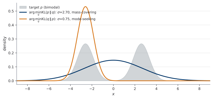
The behaviour is not an accident of this example, and the reason is visible in Equation 17. The integrand is weighted by the first argument.
\(\mathrm{KL}(p \Vert q)\) — mass-covering. The expectation is over \(p\), so the penalty is collected wherever \(p\) has mass. If \(q\) is near zero at a point where \(p\) is not, then \(\log(p/q)\) is huge there and \(p\) weights it heavily. The minimizer therefore refuses to leave any part of \(p\) uncovered, even at the cost of covering empty regions too. This direction punishes missing mass.
\(\mathrm{KL}(q \Vert p)\) — mode-seeking. Now the expectation is over \(q\), so the penalty is collected wherever \(q\) has mass. Regions where \(p\) is small are dangerous only if \(q\) goes there. The minimizer therefore keeps \(q\) inside one region where \(p\) is large and never ventures out. This direction punishes spurious mass.
One sentence on why a course about generative models cares. Training a model \(p_\theta\) by maximum likelihood turns out to be equivalent to minimizing \(\mathrm{KL}(q \,\Vert\, p_\theta)\), where \(q\) is the data distribution. Note which argument the data occupies: the first one, the one you must sample from — and sampling from the data is exactly what a dataset lets you do. UP.T1 proves that equivalence. The fact that this is the mass-covering direction, and what it costs, is a theme you will meet repeatedly.
3.4 KL between Gaussians
This is the payoff of §2. Every step below is a linear-transform or a trace manipulation, and no new idea is needed.
\[ \begin{aligned} \mathrm{KL}\big(\mathcal{N}(\mu_0, \Sigma_0) \,\big\Vert\, \mathcal{N}(\mu_1, \Sigma_1)\big) = \tfrac12\Big[ &\operatorname{tr}(\Sigma_1^{-1}\Sigma_0) \\ + &(\mu_1 - \mu_0)^\top \Sigma_1^{-1} (\mu_1 - \mu_0) \\ - &\; d + \log \tfrac{\det \Sigma_1}{\det \Sigma_0} \Big] . \end{aligned} \tag{19}\]
Derivation. Write \(p = \mathcal{N}(\mu_0, \Sigma_0)\) and \(q = \mathcal{N}(\mu_1, \Sigma_1)\). Taking logs of Equation 6, the two log-normalizers are constants and the two exponents are quadratic forms, so \[ \log \frac{p(x)}{q(x)} = \tfrac12 \log \frac{\det \Sigma_1}{\det \Sigma_0} - \tfrac12 (x - \mu_0)^\top \Sigma_0^{-1} (x - \mu_0) + \tfrac12 (x - \mu_1)^\top \Sigma_1^{-1} (x - \mu_1) . \] Take \(\mathbb{E}_{x \sim p}\) of each term. The first is constant. For the other two, use the identity that turns a quadratic form into a trace: for any symmetric \(M\) and any vector \(v\), the scalar \(v^\top M v\) equals \(\operatorname{tr}(M v v^\top)\), and the trace is linear, so it commutes with the expectation.
Second term. With \(v = x - \mu_0\) we have \(\mathbb{E}_{x \sim p}[v v^\top] = \Sigma_0\) by definition, so \[ \mathbb{E}_{x \sim p}\big[(x-\mu_0)^\top \Sigma_0^{-1} (x - \mu_0)\big] = \operatorname{tr}(\Sigma_0^{-1}\Sigma_0) = \operatorname{tr}(I_d) = d . \]
Third term. Write \(x - \mu_1 = (x - \mu_0) + (\mu_0 - \mu_1)\) and expand. The cross terms carry \(\mathbb{E}_{x \sim p}[x - \mu_0] = 0\) and vanish, so \[ \mathbb{E}_{x \sim p}\big[(x-\mu_1)^\top \Sigma_1^{-1} (x-\mu_1)\big] = \operatorname{tr}(\Sigma_1^{-1}\Sigma_0) + (\mu_0 - \mu_1)^\top \Sigma_1^{-1}(\mu_0 - \mu_1) . \]
Collecting the three pieces with their signs and the factor \(\tfrac12\) gives Equation 19; the quadratic term is symmetric in the sign of \(\mu_1 - \mu_0\). \(\square\)
Scalar corollary. With \(d = 1\), Equation 19 reads \[ \mathrm{KL}\big(\mathcal{N}(\mu_0, \sigma_0^2) \,\big\Vert\, \mathcal{N}(\mu_1, \sigma_1^2)\big) = \log \frac{\sigma_1}{\sigma_0} + \frac{\sigma_0^2 + (\mu_0 - \mu_1)^2}{2\sigma_1^2} - \frac12 . \tag{20}\]
A sanity check worth performing once: set \(\mu_0 = \mu_1\) and \(\sigma_0 = \sigma_1\) in Equation 20 and the three terms give \(0 + \tfrac12 - \tfrac12 = 0\), as Gibbs’ inequality demands.
3.5 Two more names, in passing
Two other ways of comparing distributions appear in the literature you will read. Neither is developed here; you need to recognize the names.
Total variation, \(\mathrm{TV}(p, q) = \tfrac12 \int |p(x) - q(x)|\,\mathrm{d}x\), is the largest disagreement the two distributions can have about the probability of any single event. It is a genuine metric, and it is bounded by \(1\).
The Wasserstein distance \(W_2\) measures the smallest average squared distance you must transport mass over to turn one distribution into the other. It cares about the geometry of the space, which KL does not: two narrow distributions with disjoint supports have infinite KL whether they are close together or far apart, and \(W_2\) tells them apart. \(W_2\) resurfaces near optimal-transport couplings in U3.T4.
- UP.T1 §3 proves that maximum likelihood is minimization of \(\mathrm{KL}(q \Vert p_\theta)\), the direction discussed in Section 3.3.
- U0.T3 derives a lower bound whose slack is exactly a KL term. Students who took the bootcamp have met it; students joining at the main course have not, and do not need to have.
- U3.T4 uses \(W_2\) and optimal-transport couplings.
- Equation 19 itself is the closed form behind several of the comparisons you will make in the labs.
Exercises for §3
[PS1.1.6] Work with Equation 20.
- Derive Equation 20 from Equation 19, showing the specialization of each of the four terms. (b) Fix \(\mu_0 = \mu_1 = 0\) and \(\sigma_0 = 1\), and plot or tabulate Equation 20 as a function of \(\sigma_1 \in (0, 4]\). Identify the minimum and verify it is where Gibbs’ inequality says it must be. (c) Study the two limits \(\sigma_1 \to 0\) and \(\sigma_1 \to \infty\): both give \(+\infty\), but for different reasons. State each reason in one sentence, in terms of Section 3.3. (d) Now fix \(\sigma_0 = \sigma_1 = 1\) and let \(\mu_1 - \mu_0 = \delta\). How does the divergence grow with \(\delta\)?
[PS1.1.7] Let \(p = \mathcal{N}(0, 1)\) and let \(q\) be the equal mixture \(\tfrac12 \mathcal{N}(-3, 1) + \tfrac12 \mathcal{N}(3, 1)\).
- Compute both \(\mathrm{KL}(p \Vert q)\) and \(\mathrm{KL}(q \Vert p)\) numerically, on a grid fine enough that halving the spacing does not change your third decimal place. Report the grid you used. (b) The two numbers are very different. Explain in words which direction punishes which kind of error, and which of the two errors is present here. (c) Sketch, or describe precisely, the single Gaussian that minimizes \(\mathrm{KL}(q \Vert \cdot)\) and the single Gaussian that minimizes \(\mathrm{KL}(\cdot \Vert q)\), and say which of the two you would rather have if \(q\) were a data distribution and the Gaussian were your generative model.
Slower treatment of §3, optional: (Murphy 2023) ch. 5 (§5.1 is KL); (Bishop and Bishop 2024) ch. 2.
§4 — Sampling, and change of variables in 1D
- You have a generator of \(\mathrm{Unif}(0,1)\) and a CDF \(F\) you can invert. How do you sample from \(F\)?
- \(x \sim \mathcal{N}(0,1)\) and \(y = e^x\). What is the density of \(y\)?
- In one sentence: what does “reparameterization” mean?
Answers in the footnote.4
4.1 Inverse-CDF sampling
Let \(F\) be a continuous, strictly increasing CDF on \(\mathbb{R}\), and let \(U \sim \mathrm{Unif}(0,1)\). Then \[ X \;=\; F^{-1}(U) \tag{21}\] has CDF \(F\).
Proof. Two lines. Because \(F\) is strictly increasing, \(F^{-1}(u) \le x\) holds exactly when \(u \le F(x)\). So \[ \mathbb{P}[X \le x] = \mathbb{P}\big[F^{-1}(U) \le x\big] = \mathbb{P}\big[U \le F(x)\big] = F(x) , \] the last step because \(F(x) \in [0,1]\) and \(U\) is uniform there. \(\square\)
The exponential distribution with rate \(\lambda\) has \(F(x) = 1 - e^{-\lambda x}\) for \(x \ge 0\). Solving \(u = 1 - e^{-\lambda x}\) gives \(F^{-1}(u) = -\log(1-u)/\lambda\). So \[ X = -\frac{\log(1 - U)}{\lambda}, \qquad U \sim \mathrm{Unif}(0,1) , \] is exponentially distributed with rate \(\lambda\). Since \(1 - U\) is also uniform on \((0,1)\), the version usually implemented is \(-\log(U)/\lambda\).
Equation 21 is the cleanest possible statement of what sampling is: a fixed, featureless source of randomness, pushed through a deterministic map. The distribution lives entirely in the map. Everything difficult about generative modelling is that in more than one dimension there is no CDF to invert, and the map has to be learned.
4.2 Reparameterization
The Gaussian case of the same idea has a name of its own, and you have already seen the formula as Equation 7.
\[ x \;=\; \mu + \sigma \varepsilon , \qquad \varepsilon \sim \mathcal{N}(0,1) \qquad\Longrightarrow\qquad x \sim \mathcal{N}(\mu, \sigma^2) . \tag{22}\]
Say what Equation 22 does in words, and say it in this exact form:
Sampling is pushing a fixed noise source through a deterministic map.
Read it again with \(\mu\) and \(\sigma\) replaced by the output of a neural network, and you have a generative model. Read it again with the map replaced by the solution of a differential equation, and you have the second half of this course. The source never changes; the map is what you learn.
There is a second reason Equation 22 matters, and it is computational. Because \(\varepsilon\) does not depend on \(\mu\) or \(\sigma\), the derivative of \(x\) with respect to those parameters is available: \(\partial x/\partial \mu = 1\) and \(\partial x / \partial \sigma = \varepsilon\). Randomness that sits outside the parameters can be differentiated through. Randomness that sits inside them cannot. That distinction is what makes gradient-based training of a sampler possible at all.
4.3 Change of variables in one dimension
Let \(X\) have density \(p_x\), let \(g\) be differentiable and strictly monotone, and set \(Y = g(X)\). Then the density of \(Y\) is \[ p_y(y) \;=\; p_x\big(g^{-1}(y)\big)\, \left| \frac{\mathrm{d}\,g^{-1}}{\mathrm{d}y}(y) \right| . \tag{23}\]
Derivation, via the CDF. Take \(g\) increasing, so that \(g(X) \le y\) holds exactly when \(X \le g^{-1}(y)\). Then \[ F_y(y) = \mathbb{P}[Y \le y] = \mathbb{P}\big[X \le g^{-1}(y)\big] = F_x\big(g^{-1}(y)\big) . \] Differentiate in \(y\), using the chain rule on the right: \[ p_y(y) = p_x\big(g^{-1}(y)\big) \cdot \frac{\mathrm{d}\,g^{-1}}{\mathrm{d}y}(y) . \] For decreasing \(g\) the same computation runs with the inequality reversed, producing \(1 - F_x(g^{-1}(y))\) and hence a minus sign, which the absolute value in Equation 23 absorbs. \(\square\)
The absolute value is the whole content. The derivative \(|\mathrm{d}g^{-1}/\mathrm{d}y|\) measures how much the map stretches or compresses the line near \(y\). Where \(g\) stretches an interval, it spreads the same mass over a wider range, so the density there must go down by exactly that factor. Probability mass is conserved; density is not. Figure 4 shows this with the two intervals and the two shaded areas.
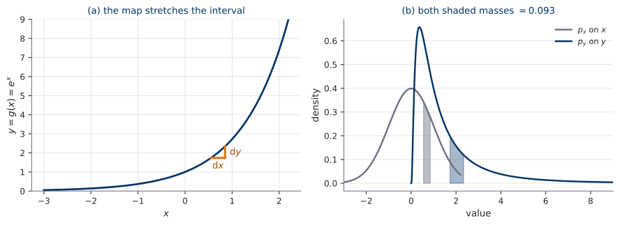
Figure 4 makes the claim at one place, with one interval. The claim itself is about every place, and the animation below is that sweep. An interval of fixed width \(\mathrm{d}x = 0.300\) is carried along the line, and two numbers are displayed the whole time: the mass under \(p_x\) over the interval, and the mass under \(p_y\) over its image. They stay locked — the two agree to better than \(10^{-9}\) at every point of the sweep, which the precompute asserts before the scene is allowed to draw anything:
The sweep deliberately crosses the place where \(\mathrm{d}g^{-1}/\mathrm{d}y\) equals \(1\). To the left of it the map compresses: the image interval is narrower and the density over it is taller. To the right it stretches: the image is wider and the density is shorter. The local factor runs from about \(0.24\) to about \(4.28\) across the sweep, and the mass never moves. One interval is an instance; this is the claim.
Carry the resulting mental object forward, because it is the one U1 needs. In \(d\) dimensions this local stretching factor becomes a Jacobian determinant, and a reader who has watched a factor vary along a line has the right picture for that. A reader who has seen one rectangle does not.
Let \(x \sim \mathcal{N}(0, 1)\) and \(y = g(x) = e^x\), so \(g^{-1}(y) = \log y\) for \(y > 0\) and \(\mathrm{d}g^{-1}/\mathrm{d}y = 1/y\). Then Equation 23 gives \[ p_y(y) \;=\; \mathcal{N}(\log y; 0, 1) \cdot \frac{1}{y} \;=\; \frac{1}{y\sqrt{2\pi}} \exp\!\big(-\tfrac12 (\log y)^2\big) , \qquad y > 0 , \] which is the standard log-normal density. Note that the factor \(1/y\) is not cosmetic: without it the expression does not integrate to \(1\), and it is what makes the density fall away near \(y = 0\) even though \(\log y\) is heading toward the middle of the Gaussian.
In \(d\) dimensions, the stretching factor \(|\mathrm{d}g^{-1}/\mathrm{d}y|\) becomes the absolute determinant of a Jacobian matrix, \(|\det J_{g^{-1}}(y)|\). That theorem opens U1, and its proof is assigned as PS1.3. It is not proved here, and the one-dimensional case above is not a proof of it.
4.4 Two directions, one map
There is a tension hidden in Equation 23, and it is worth seeing now, because a whole unit of this course is organized around it.
To sample, you need \(g\): draw \(x\) from the simple source and evaluate \(g(x)\). You never need the inverse.
To evaluate the density at a given point \(y\), you need \(g^{-1}\), because Equation 23 asks you to find the point that mapped there. You also need the derivative of that inverse.
In one dimension a monotone \(g\) gives you both, and there is no difficulty. In \(d\) dimensions the two requirements pull against each other: a map that is cheap to evaluate forwards may be expensive or impossible to invert, and the determinant of its Jacobian may cost as much as a matrix factorization. U1 is largely the story of designing maps that keep both directions affordable, and of what expressive power that design costs. U2 removes the constraint by a different route entirely.
- U1.T1 proves the multivariate version of Equation 23, with the Jacobian determinant, and PS1.3 assigns the proof.
- U1.T2 is about the sampling-against-density duality of
- Equation 22 is used in every lab in the course, wherever a sample must be differentiated through.
Exercise for §4
[PS1.1.8] Let \(x \sim \mathcal{N}(0, 1)\) and \(y = \tanh(x)\).
- Derive the density of \(y\) on \((-1, 1)\) using Equation 23, giving both \(g^{-1}\) and its derivative explicitly. (b) Evaluate your density at \(y = 0\) and at \(y = 0.9\), and confirm numerically that it integrates to \(1\) over \((-1,1)\). (c) Describe the behaviour of the density as \(|y| \to 1\), and explain which factor in Equation 23 is responsible. (d) You will eventually implement such a map in floating-point arithmetic. State, in two sentences, what goes wrong numerically near \(|y| = 1\) and what quantity you would compute in log-space to avoid it.
Slower treatment of §4, optional: (Murphy 2023) §2.5, “Transformations of random variables”. (Lipman et al. 2024) states the multivariate change of variables, with the Jacobian matrix, already in the notation of this course — that is where Section 4.3 is heading, and it is U1’s material rather than this section’s.
§5 — Notation drill
- In \(\mathbb{E}_{x \sim p}[f_\theta(x)]\), which symbols are integrated over and which are held fixed?
- Rewrite \(\mathbb{E}[\|f(y) - x\|^2]\) so that a reader cannot mistake what is random.
- In this course, is \(t = 0\) noise or data?
Answers in the footnote.5
This section teaches no probability. It teaches the grammar in which the rest of the course is written, and it exists because the single most common way to misread a paper in this field is to misread an expectation.
5.1 Reading an expectation with subscripts
Three examples, each one step more nested than the last.
One distribution. \[ \mathbb{E}_{x \sim q}\big[\, \|x\|^2 \,\big] . \] One variable is drawn, from the data distribution \(q\). The result is a number.
Two distributions, drawn independently. \[ \mathbb{E}_{x_0 \sim p_0,\; x_1 \sim q}\big[\, \|x_1 - x_0\|^2 \,\big] . \] Two variables are drawn, one from the standard Gaussian source and one from the data, and the comma means they are drawn independently. The result is again a number.
A chain: draw, then draw conditionally on what you drew. \[ \mathbb{E}_{t,\; x_1 \sim q,\; x \sim p_t(\cdot \mid x_1)}\big[\, \ell(x, x_1, t) \,\big] . \tag{24}\] Read Equation 24 from left to right, because the order is meaningful. First \(t\) is drawn. Then \(x_1\) is drawn from the data distribution. Then \(x\) is drawn from a density that depends on both of the previous draws — that is what the vertical bar and the dot are for: \(p_t(\cdot \mid x_1)\) is a density in its first argument, indexed by \(t\), conditioned on \(x_1\).
It is here as a pattern to recognize, and nothing more. You will see this exact shape weekly from U3 onwards. What \(p_t\) is, where it comes from, and why anyone would want it, are questions this primer does not answer and must not: \(p_t\) is some time-indexed family of densities, and the details belong to U3. The grammar is the lesson here; the content comes later.
5.2 The rewriting game
Below are three expressions of the kind that appear in real papers. Each is ambiguous. Each is followed by a standard-form rewriting and a one-line diagnosis of what the ambiguity was.
Sloppy 1. \[ \mathcal{L}(\theta) = \mathbb{E}\big[\, \|f_\theta(y) - x\|^2 \,\big] . \]
Standard form. \[ \mathcal{L}(\theta) = \mathbb{E}_{(x, y) \sim p}\big[\, \|f_\theta(y) - x\|^2 \,\big] . \]
Diagnosis. The bare \(\mathbb{E}\) does not say whether the pair is drawn jointly or the two are drawn independently, and the difference is not small: under independent draws the loss is minimized by the constant \(\mathbb{E}_{x \sim p}[x]\), and the function \(f_\theta\) has nothing to learn.
Sloppy 2. \[ \mathcal{L}(\theta) = \mathbb{E}_{x, t}\big[\, \|u_t^\theta(x) - u_t(x)\|^2 \,\big] . \]
Standard form. \[ \mathcal{L}(\theta) = \mathbb{E}_{t \sim \mathrm{Unif}[0,1],\; x \sim p_t}\big[\, \|u_t^\theta(x) - u_t(x)\|^2 \,\big] . \]
Diagnosis. The subscript named the variables but not their distributions. Two questions were left open, and both matter: how \(t\) is distributed on \([0,1]\), and — the important one — that \(x\) is drawn from a density that depends on \(t\). Writing \(x \sim p_t\) makes the dependence visible; writing \(\mathbb{E}_{x,t}\) hides it.
Sloppy 3. \[ \mathcal{L}(\theta) = \mathbb{E}_{x_1}\big[\, \|u_t^\theta(x) - u_t(x \mid x_1)\|^2 \,\big] . \]
Standard form. \[ \begin{aligned} \mathcal{L}(\theta) = \mathbb{E}_{t \sim \mathrm{Unif}[0,1],\; x_1 \sim q,\; x \sim p_t(\cdot \mid x_1)} \big[\, \|u_t^\theta(x) - u_t(x \mid x_1)\|^2 \,\big] . \end{aligned} \]
Diagnosis. Two free symbols, \(t\) and \(x\), appeared in the integrand without appearing in the subscript. An expression like that is not a number: it is a function of whatever was left unbound, and the reader cannot tell which. The repair is mechanical, and it is the rule below.
Every symbol inside the brackets is either bound — it appears in the subscript, with a distribution — or it is a parameter, and the expression is a function of it. There is no third case. Before you write \(\mathbb{E}\), list the symbols inside and classify every one.
5.3 The four rules, verbatim
These are copied from the course notation standard, and they are binding on everything you write in this course, including problem sets.
- Never write a loss without explicit sampling subscripts on \(\mathbb{E}\).
- Never use the diffusion time arrow outside the Rosetta Stone.
- When quoting a source that uses different notation (for example \(v_t\) for velocity, \(x_T\) for noise, \(\rho\) for density), translate silently to the course standard; add a footnote only when the discrepancy is pedagogically instructive.
- The Lemma is always cited by name (“the projection Lemma”, UP.T1) when invoked.
Rules 2 and 4 name things you have not met. That is intended: you will meet them, and when you do, the rule is already in force. Rule 1 is the one that applies to you today, in the exercise below.
Everywhere, without exception, starting with UP.T1. Rule 4 is the naming convention for the result proved in that session. Rule 2 becomes live in U3.T1, and the Rosetta Stone it mentions is the living handout that grows through the U3 detours.
Exercise for §5
[PS1.1.9] Rewrite each expression below into the standard form of this course. For each, list every symbol inside the brackets and classify it as bound (naming the distribution you chose, and justifying the choice in a few words) or parameter.
\(\displaystyle \mathcal{L}(\theta) = \mathbb{E}\big[\log p_\theta(x)\big]\), intended as the objective of maximum-likelihood training on a dataset drawn from \(q\).
\(\displaystyle \mathcal{L}(\phi, \theta) = \mathbb{E}_{z}\big[\log p_\theta(x \mid z)\big] - \mathrm{KL}\big(q_\phi(z \mid x) \,\Vert\, p(z)\big)\), intended as a per-example objective for a latent-variable model.
For part (b), state additionally whether the expression is a number or a function of \(x\), and say what would have to be added to make it the other one.
Appendix A — The course notation standard
This table is the canonical symbol table for every artifact of this course. It is reproduced here unchanged, and it is the first place to look whenever a symbol is unfamiliar.
The table is a reference for the whole course, not a summary of this page. Rows for \(p_t\), \(\psi_t\), \(u_t\), \(u_t^\theta\) and \(s_t\) name objects that are defined in U2 and U3, and nothing on this page depends on them. They are listed so that the standard is fixed from the first day and never renegotiated. Read the table now for the rows you recognize; return to it later for the rest.
Time and direction. \(t \in [0,1]\); \(t = 0\) is noise, \(t = 1\) is data. All diffusion material is translated into this arrow; the diffusion-native arrow appears only in the Rosetta Stone, with explicit translation rules (\(s = 1 - t\) and schedule remappings).
| Object | Symbol | Notes |
|---|---|---|
| Data distribution | \(q\), samples \(x_1 \sim q\) | on \(\mathbb{R}^d\) |
| Encoder / variational distributions | \(q_\phi(z \mid x)\) | subscript mandatory; unsubscripted \(q\) is always the data distribution |
| Source / noise | \(p_0 = \mathcal{N}(0, I_d)\), samples \(x_0\) | |
| Probability path | \(p_t\) | marginal path, \(p_0 \to q\) ideally at \(t = 1\) |
| Conditional path | \(p_t(x \mid x_1)\) | designer’s choice |
| Flow map | \(\psi_t\) | \(\psi_0 = \mathrm{id}\) |
| Marginal velocity | \(u_t(x)\) | generates \(p_t\) via the continuity equation |
| Conditional velocity | \(u_t(x \mid x_1)\) | generates \(p_t(\cdot \mid x_1)\) |
| Learned field | \(u_t^\theta(x)\) | network; never \(v_\theta\) in our materials |
| Score | \(s_t(x) = \nabla_x \log p_t(x)\) | |
| Gaussian path schedule | \(\alpha_t, \sigma_t\) | \(x_t = \alpha_t x_1 + \sigma_t x_0\) for Gaussian paths |
| Noise parametrization | \(\varepsilon\)-prediction \(\varepsilon_\theta\) | appears in D2 and the Rosetta Stone |
| Jacobian | \(\partial f / \partial x\) or \(J_f(x)\) | matrix of partials |
| Divergence | \(\nabla \cdot f = \operatorname{tr}(\partial f/\partial x)\) | both notations declared equal once, then \(\nabla \cdot\) |
| KL divergence | \(\mathrm{KL}(p \,\Vert\, q)\) | double bar |
| Gaussian | \(\mathcal{N}(x; \mu, \Sigma)\) | |
| Expectations | \(\mathbb{E}\) with explicit sampling subscripts | for example \(\mathbb{E}_{t,\, x_1 \sim q,\, x \sim p_t(\cdot \mid x_1)}\) — mandatory in every loss |
| Losses | \(\mathcal{L}_{\mathrm{FM}}(\theta)\), \(\mathcal{L}_{\mathrm{CFM}}(\theta)\), \(\mathcal{L}_{\mathrm{DSM}}(\theta)\) | |
| Dimension | \(d\) | |
| ODE / SDE | \(\mathrm{d}x = u_t(x)\,\mathrm{d}t\); \(\mathrm{d}x = f_t(x)\,\mathrm{d}t + g_t\,\mathrm{d}W\) |
\(W\) standard Wiener |
What to do next
You have five things to hand in and one live session to prepare for.
- Do the nine exercises. They are PS1.1, and they are graded. Together they take a few evenings, not one.
- Keep the toolkit sheet. The two-page extract of §2 is the sheet you will actually reach for during U3. Print it, or keep the page open.
- Copy Equation 16 somewhere permanent. You were told why, roughly.
- Read the four rules of Section 5.3 once more before the first live session. Rule 1 will be enforced on every problem set.
- Come to UP.T1 knowing Equation 5 informally. That session proves it, and then proves the result the whole course rests on out of it.
References
Footnotes
- \(p(y) = \int p(x, y)\,\mathrm{d}x\) and \(p(x \mid y) = p(x,y)/p(y)\) wherever \(p(y) > 0\). (2) Independent, yes; independent given \(Z\), no — knowing \(Z\) makes \(X\) determine \(Y\). This is the reverse of the example in Section 1.2, and both directions happen. (3) \(\mathbb{E}[X] = 1.5\), by averaging the two conditional means.
- \(\mathcal{N}(A\mu + b,\; A \Sigma A^\top)\). (2) Yes, and no — the conditional covariance does not depend on the value of \(x_b\), which is a special property of Gaussians and the reason they are so convenient. (3) \((x - A^{-1}b)^\top A (x - A^{-1}b) - b^\top A^{-1} b\).
- \(\mathrm{KL}(p \Vert q) = \mathbb{E}_{x \sim p}[\log p(x) - \log q(x)]\).
- No, and no — it is asymmetric, and it is non-negative, which Section 3.2 proves. (3) Minimizing \(\mathrm{KL}(q \Vert p)\) over \(q\) picks one hump; minimizing \(\mathrm{KL}(p \Vert q)\) spreads across both. See
- \(X = F^{-1}(U)\) with \(U \sim \mathrm{Unif}(0,1)\); see Equation 21.
- \(p_y(y) = \mathcal{N}(\log y; 0, 1)/y\) for \(y > 0\), the log-normal; see Equation 23. (3) Writing a random draw as a deterministic function of a fixed, simple noise source.
- \(x\) is integrated over; \(\theta\) is a parameter, and the value of the expression depends on it. (2) Any unambiguous version is acceptable, for example \(\mathbb{E}_{(x,y) \sim p}[\|f(y) - x\|^2]\) — what is not acceptable is leaving it as given. (3) \(t = 0\) is noise and \(t = 1\) is data, always, everywhere in this course.