U0.L4 — U-Net Skeleton and Eval Harness
Session U0.L4 · date: see calendar-map
This is the highest-leverage session of the bootcamp, and the reason is not that the material is hard. It is that today you write two pieces of code that the rest of the course imports without modification. The network you assemble is the one U3 trains, conditions and samples from. The harness you write is the instrument every later number in this course is measured with. Both interfaces are frozen at the end, and after that a change to either is a breaking change.
That framing decides how the session is scaffolded. The primitive blocks — the residual block with its modulation, the attention block, the two resampling layers — are given to you complete, and they are short enough that you are asked to read them. What you write is the part that transfers: the wiring, the conditioning path, and the metrics. Transcribing convolution boilerplate under time pressure teaches nothing, and the artifacts have to be correct, because everything else sits on them.
The previous theory session (U0.T4) built all of this on paper: the U-Net’s anatomy, the sinusoidal ladder, FiLM modulation, the embedding-sum rule, the Fréchet distance and its three caveats. None of it is re-derived here. Today it becomes code, and the caveats become asserts.
Format. Scripts and a package, not a notebook — these two artifacts live in common/, beside the hygiene-stack you wrote in U0.L2, because that is where importable code belongs. A driver notebook (lab-u0l4.ipynb) holds the checks and the pictures.
Every number in these notes was measured. The runs behind the figures are in scripts/python/fig_u0_l4_eval.py, seeded, and the values are recorded in scripts/python/_outputs/u0l4_eval.json. One of this session’s plans turned out to be self-contradictory when it was run, and Section 3 reports it as it came out.
Standing reference for the architecture and the evaluation material: Bishop and Bishop (Bishop and Bishop 2024). The U-Net is (Ronneberger, Fischer, and Brox 2015), the modulation mechanism is (Perez et al. 2018), and the metric is (Heusel et al. 2017).
A · The contracts
Reused in: U3.L2, U3.L3, U1.L2, PS1.4, PS0 — that is, everywhere.
Why a contract comes before any code
Every previous lab ended by freezing an interface. This one starts by freezing two, because the freeze is the deliverable. Four later sessions import these names, and they will import them from a written specification rather than from whatever the code happens to do. So the specification is written first, and the code is then made to satisfy it.
UNet(in_ch, base_ch, ch_mults, attn_resolutions, num_classes=None)

forward(x: (B, C, H, W) float,
        t: (B,)         float in [0, 1],
y: (B,) long, optional) -> (B, C, H, W)tis always a(B,)tensor of floats in \([0,1]\). This is the FM time arrow at code level: \(t=0\) is noise, \(t=1\) is data. Any later code that needs a different time variable converts outside this network.yis optional, and its pathway exists only whennum_classesis given. The label embedding is summed into the time embedding (U0.T4’s embedding-sum rule), never concatenated.- The output has the input’s shape. It is a per-pixel quantity.
Point 1 is the one worth dwelling on. It is a single line in a signature, and it is what keeps the diffusion dialect out of this codebase. Every reference implementation you will read takes an integer timestep counting down from a thousand; every one of them therefore invites you to write \(\beta_t\), \(\bar\alpha_t\) and a reversed arrow into your own code, one function at a time, until the codebase speaks two languages. The assert in forward refuses the first step of that.
Point 2 is an act of planning. The class-conditional pathway is built today and deliberately unused. U3.L3 will want it, and when it arrives it should need no architectural surgery — only the guidance logic, which is not here.
common/eval.py
  FeatureExtractor            # protocol: name, preprocessing, dim, __call__
    MNISTFeatures             # course classifier, pinned weights
    InceptionV3Features       # torchvision, for CIFAR and beyond

  ref_stats(loader, extractor)              -> RefStats(mu, Sigma, ...)
  fid(samples, ref, extractor)              -> float
  bpd(total_log_likelihood_nats, num_dims)  -> float
  panel(model_sample_fn, eps_bank, path)    -> figure
The comparability rule, printed in the module’s docstring and enforced by its code: an FID is not a property of a model, it is a property of a model and a measurement protocol. Two values are comparable only when the extractor, the preprocessing and the sample count all agree.
The extractor decision, settled
U0.T4 left caveat (iii) open: the extractor decides what “similar” means, and the standard extractor is an ImageNet classifier whose features were shaped by a task and a dataset that MNIST resembles not at all. The course resolves it here, and the resolution is binding.
MNIST evaluations use MNISTFeatures — a small convolutional classifier trained on MNIST itself, weights pinned and committed, penultimate layer (128 units) as the feature space. InceptionV3Features is reserved for CIFAR and beyond.
The weights are pinned rather than trained by you, and the reason is the comparability rule one level up. Every FID in this course must be comparable across students, across sessions and across machines, which is true only if everyone measures in the same feature space. The training script ships with the course so the choice is inspectable — but running it again produces a different extractor, and therefore a different, self-consistent, incomparable scale.
scripts/python/train_mnist_features.py, seed 0, eight epochs, best-on-validation selection. The shipped weights reach 99.22 % validation accuracy on a held-out ten thousand images. The file records a SHA-256 of the weights beside the accuracy, and MNISTFeatures carries both, so any number this course reports can be traced back to the extractor that produced it.
One deliberate inconsistency to name before someone spots it. The extractor uses BatchNorm, which the recipe card bans from the U-Net. The law is about the failure, not about the layer: BatchNorm is forbidden in a generative model because that model is sampled one example at a time, so batch statistics would make one sample depend on the others. A classifier used only in eval() runs on frozen running statistics and depends on no batch at all.
B · Assembling the U-Net
Reused in: every time-conditioned model in the course.
The build map is the U-Net anatomy diagram of U0.T4 — the same picture, on the screen for the whole part. Every box in it is something you wire.
TODO 1 — the ladder
The frozen spec, from the sinusoidal-ladder definition of U0.T4. For t a (B,) float tensor in \([0,1]\) and an even width dim, with half = dim // 2:
freqs = torch.exp(-math.log(10000.0) * torch.arange(half) / half)
arg   = (1000.0 * t)[:, None] * freqs[None, :]
emb   = torch.cat([torch.sin(arg), torch.cos(arg)], dim=-1)
The factor \(1000\) is the only rescale and it is deliberate: it makes this from-scratch ladder produce the same numbers as the DiT and ADM reference implementations, so that a later cross-check against a library reports real bugs instead of convention differences. Outside this one function, \(t\) is a float in \([0,1]\) everywhere.
TODO 2 — the wiring, and the shape table
This is the honest difficulty of the session, and it is bookkeeping rather than insight. The encoder pushes an activation onto a stack at every step. The decoder pops one at every step and concatenates it on the channel axis before its residual block runs. The decoder’s input width therefore depends on what the encoder happened to push, and a table is the only way to keep it straight.
The reference configuration — in_ch=1, base_ch=64, ch_mults=(1, 2, 2), attn_resolutions=(7,) — builds this ladder:
| Level | Resolution | Channels | Attention |
|---|---|---|---|
| 0 | \(28 \times 28\) | 64 | — |
| 1 | \(14 \times 14\) | 128 | — |
| 2 | \(7 \times 7\) | 128 | yes |
| bottleneck | \(7 \times 7\) | 128 | yes |
Attention appears only at the bottom, and U0.T4’s cost argument is the reason: the cost is quadratic in the number of positions, so \(7 \times 7\) costs about \(1/256\) of what \(28 \times 28\) would.
The decoder gets one extra residual block per level. That is not a stylistic choice: the level’s last skip is the one the downsampling layer pushed, and it needs a block of its own to be consumed. A decoder with the same block count as its encoder leaves one skip on the stack, and the failure is a shape error deep inside the last level rather than anything legible.
The stack is easier to watch than to read about. The animation below runs it twice. The first run has the extra block, and the stack ends empty. The second run has the encoder’s block count, and it does not reach the end at all: a pop arrives with the decoder at one resolution and the tile at another, and that mismatch is the error you would actually see. The tiles still unread are counted on screen after it stops:
Three things pass before you continue.
- Shapes. A forward pass at \(28 \times 28\) returns \(28 \times 28\); the same model on a \(14 \times 14\) input returns \(14 \times 14\).
- Parameter count within 5 % of the reference: 6 946 881 unconditional, 6 947 521 with a ten-class pathway. The class pathway costs 640 parameters — a table of ten vectors of width 64 — which is the embedding-sum rule’s whole price.
- The reading question. The provided blocks call
num_groups(channels)rather than passing32. What does it return for 64, for 128, and for 1, and why is the answer not always 32?
The answer to the third: GroupNorm requires the group count to divide the channel count, so hard-coding 32 crashes the moment base_ch is not a multiple of it. num_groups returns the largest admissible count at or below 32 — so 32, 32 and 1 for those three widths.
TODO 3 — the conditioning path
The ladder’s output has width base_ch. A small multilayer perceptron lifts it to d_emb (four times base_ch, so 256 here), and that vector reaches every residual block at every resolution, where a zero-initialized linear map turns it into one scale and one shift per channel.
The label table has the ladder’s width, not d_emb, because the sum happens before the projection:
\[ c = \mathrm{emb}(t) + \mathrm{emb}(y) \;\longrightarrow\; \text{MLP} \;\longrightarrow\; (\gamma, \beta) . \]
One projection, whatever the number of conditioning signals. Concatenating instead would grow the modulation path every time a signal was added, and would need a wider projection in every block.
C · Is the conditioning alive?
Reused in: every time-conditioned model henceforth. These become the course’s standard checks.
A wired network that runs is not a working network. The three rituals below are cheap, they take under a minute together, and each of them has caught a real bug in this course’s own code. From here on they run whenever a conditioned model is built.
But they cannot all run at the same moment, and finding out why is the most useful thing in this part.
The plan for this part was self-contradictory
The session plan asked for two checks, in this order:
- Ritual 1 — sensitivity to \(t\). Fix \(x\), sweep \(t\) over \([0,1]\), and assert that the outputs differ.
- Ritual 2 — the zero-init check. At initialization, assert that the output is approximately zero, because the final convolution is zero-initialized.
Run both at initialization and they contradict each other. The recipe card’s zero-initialization does not make the output approximately zero; it makes it exactly zero, bit for bit, for every \(t\). A network whose output is identically zero cannot distinguish two times, so ritual 1’s assert must fail — not because the conditioning is broken, but because there is nothing yet to be sensitive with.
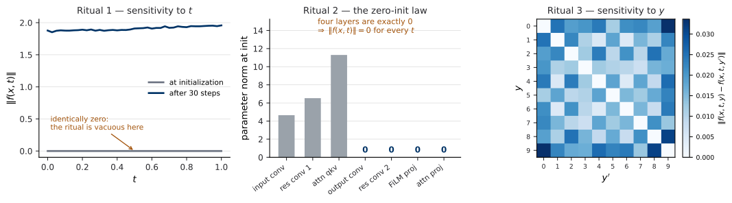
The left panel of Figure 1 is that finding. The flat grey line is not a network with dead conditioning; it is a network that is the zero function, which is exactly what ritual 2 asks it to be.
This is the second time the course has met this shape. In U0.L3 the gradient-check ritual had the same defect: with zero-initialized heads the gradient into the encoder body is exactly zero, so the check reported a perfect relative error of \(0.0\) while measuring nothing. The rule that comes out of both:
A check that asserts a network does something cannot run at initialization if the initialization is designed to make the network do nothing. Run the zero-init check first, at initialization; then move the parameters; then run everything else.
Moving the parameters is not training. Thirty optimizer steps against random targets — no dataset, no generative objective, result discarded — is enough to leave the zero function, and it is what the session’s wake_up helper does. The U-Net is not trained today; its first real training is U3.L2, by design.
The three rituals, measured
Ritual 2 — the zero-init law. At initialization, four norms are exactly zero: the output convolution, the last convolution of every residual branch, every FiLM projection, and every attention output projection. Every other layer — the input convolution, each residual branch’s first convolution, the attention query-key-value projection — is initialized normally, and the middle panel of Figure 1 plots the two groups side by side, because the contrast is the message. That the four are zero makes the untrained network the zero field. It is not a coincidence but a law of the recipe card, and the middle panel of Figure 1 reports it as measured rather than as intended.
Ritual 1 — sensitivity to \(t\). After the wake-up, \(\|f(x,t)\|\) varies over the sweep with a relative spread of about 5.6 %. The assert is that the spread is strictly positive: a network that returns the same thing at \(t = 0\) and \(t = 1\) has a conditioning path that is wired to nothing, which is the single most common way a time-conditioned model fails silently. It trains, the loss falls, and the model is a \(t\)-independent average of what it should have learned.
Ritual 3 — sensitivity to \(y\). With the class pathway on, the outputs at ten different labels are pairwise distinct at fixed \((x, t)\): the pairwise distances run from about \(0.004\) to about \(0.034\). The right panel of Figure 1 shows the whole matrix, and the thing to notice is that it is not near-constant — the label reaches the computation with a different effect for each class, which is what an embedding table should do.
The gradient-check ritual. Finite differences against autograd on one FiLM projection weight, in the U0.L1 and U0.L3 lineage, relative error of order \(10^{-7}\). And, because a check that has never failed is not known to work, the same comparison is re-run against a deliberately doubled gradient, where it must fail — it reports a relative error of \(0.5\).
The split test, the garbage test and the two VAE values reproduce exactly between runs of the measurement script. The three ritual numbers above do not: they move in their last digits, and the reason is that they come from a thirty-step optimization on a GPU, whose kernels are not bit-deterministic unless you ask.
That is the course convention stated as a consequence rather than a rule. Determinism on an accelerator is opt-in — torch.use_deterministic_algorithms(True) and the matching cuDNN setting buy it, and they cost throughput. A seed alone does not. So a number that has to be quoted is either measured on a deterministic path or quoted to the precision it actually holds, and claiming more than that is the failure this paragraph exists to prevent.
D · The evaluation harness
Reused in: U1.L2 and PS1.4 (bpd), U3.L2 and U3.L3 (fid, ref_stats, panel), PS0 (all).
U0.T4 wrote the definitions. This part writes the code, and the interesting part of writing it is that two of the three caveats become properties of the program rather than things to remember.
TODO 4 — reference statistics, and why float64
ref_stats pushes a loader through the extractor and returns the mean and covariance of the features. It runs once over a large reference set, and it caches to disk, because the reference side of an FID does not change between models.
Two decisions carry the teaching.
The accumulation is in float64, and this is not fastidiousness. A covariance is a sum of products of numbers whose magnitudes differ by orders of magnitude. In float32, small contributions are lost to rounding against a growing sum, and the resulting matrix can fail to be positive semi-definite. The failure then surfaces two functions away, inside a matrix square root, as a complex number nobody expected.
The cache key is caveat (i), written as a filename. The cached file is named for the dataset, the extractor and the preprocessing:
refstats__mnist-test__mnist-cnn-v1__01-float-28x28.npzA key that omitted the preprocessing would serve statistics from the wrong pipeline on a cache hit — silently, permanently, and exactly as the caveat warns. Writing the key this way makes that impossible rather than unlikely.
TODO 5 — the Fréchet distance, and the imaginary part
The formula is U0.T4’s, transcribed:
\[ \begin{aligned} \mathrm{FID} \;=\;& \lVert \mu_r - \mu_g \rVert^2 \\ &+ \operatorname{Tr}\!\left( \Sigma_r + \Sigma_g - 2 (\Sigma_r \Sigma_g)^{1/2} \right). \end{aligned} \]
The matrix square root is where implementations go wrong, and the failure is worth naming because it is invisible. scipy.linalg.sqrtm works on general matrices and returns a complex array. On a product of two covariance matrices the true root is real, but floating-point error decorates it with a tiny imaginary component. The standard fix is to call .real and move on.
That fix is wrong, and only wrong sometimes. Calling .real unconditionally also discards a large imaginary part, and a large one means the input was not positive semi-definite — a genuine upstream bug, usually a covariance accumulated in float32. So the harness truncates only after measuring what it is truncating:
if imag_max / real_scale > 1e-3:
    raise ValueError("the input is not positive semi-definite — "
"check that the covariances were float64")TODO 6 — bits per dimension
Mechanically, the definition of U0.T4:
\[ \mathrm{BPD} = -\frac{\mathbb{E}_{x \sim q}[\log p_\theta(x)]}{d \log 2}, \]
with the argument given in nats and \(d = 784\) for MNIST. Lower is better, and the quantity is a compression rate.
One thing is deliberately missing. A likelihood on continuous space compared against discrete pixel data needs a dequantization correction before the number means anything across papers. It is added when the course first uses bits per dimension, in U1. Today the function is mechanical, and the docstring carries the marker so that nobody later mistakes its absence for a decision that was made.
TODO 7 — the panel
panel formalizes the trick U0.L3 used by hand: a fixed bank of noise, drawn once and reused at every evaluation. Two panels from two checkpoints then differ because the model changed, and not because the noise did. Without it, a visual comparison across epochs is a comparison of two unrelated draws, and every real change smaller than the sampling noise is invisible.
E · Calibrating the instrument
Reused in: every FID this course reports.
A metric is not trusted because it is implemented. It is trusted because it was checked against cases whose answer is known. Three such cases, and the three numbers they produce go into every student’s session log:
- the split test — MNIST cut in half, where the true answer is zero;
- the sample-count curve — the same split at several sample counts;
- the garbage test — noise images against MNIST.
The split test: the answer is zero, and the measurement is not
Take the MNIST training split, cut it in half at random, and score one half against the other. The two halves are independent draws from one distribution, so the true FID is exactly zero. Everything measured is bias.
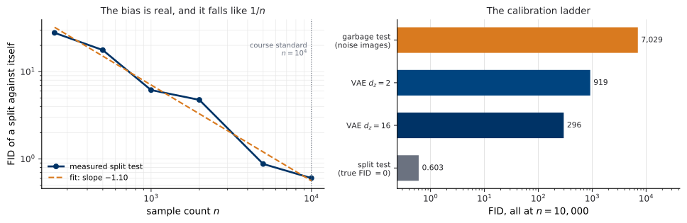
At the course standard of ten thousand samples, the harness reports 0.603. It is small, and it is not zero, and it is not noise: the left panel of Figure 2 measures it at six sample counts, and it falls monotonically from \(27.8\) at \(n = 250\) to \(0.603\) at \(n = 10^4\), with a fitted log-log slope of \(-1.10\). That is caveat (ii) as a law rather than a warning — the bias falls like \(1/n\).
The individual points scatter around that line rather than sitting on it, and the scatter is honest: each count is one draw of samples, not an average over draws, so a point carries the sampling variability of a single measurement on top of the bias it is estimating. U0.T4 drew the same law on a synthetic Gaussian, where the curve is visibly cleaner. Real features are noisier, and the law survives it.
This is where the course’s reporting rule comes from, and it is now a rule rather than a preference:
Report FID at a fixed sample count — ten thousand for MNIST — or report the whole curve. Never compare two values measured at different counts.
U0.T4 measured what the rule buys. Because the bias is systematic, at equal \(n\) it lands on both models and cancels, so the ranking survives; at unequal \(n\) it does not cancel, and the ranking inverts exactly when the difference in bias exceeds the true gap.
The garbage test: the instrument has range
Score ten thousand uniform-noise images against MNIST. The harness reports 7028.6 — about eleven thousand times the split test. That ratio is the point. An instrument whose reading barely moves between “the same distribution” and “no distribution at all” cannot resolve anything in between, and the right panel of Figure 2 is the whole span, on one axis, before any of it is trusted.
The payoff: the eye test becomes a number
In U0.L3 you trained two VAEs on MNIST, at \(d_z = 2\) and \(d_z = 16\), and looked at their samples. The wider one looked better. “Looked better” is where the course has been until now.
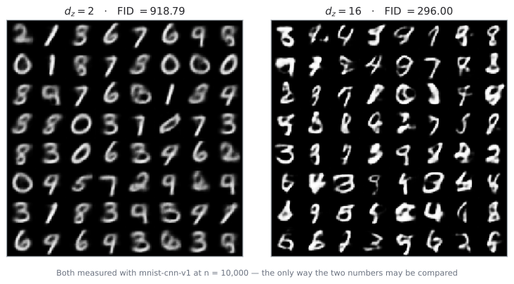
Figure 3 shows both, and the measured values are 918.8 at \(d_z = 2\) and 296.0 at \(d_z = 16\), both at ten thousand samples with the pinned extractor. The eye test was right, and now it has a size: the narrower model scores 3.1 times worse.
Before reading anything into the size of those numbers: the absolute scale of an FID is a property of the extractor, not of the models. These features are 128 unnormalized units from a small MNIST classifier, and a value of \(296\) here is not comparable with any published MNIST FID, all of which use Inception features on a different scale. Within this course’s protocol the values order models correctly and their ratios are meaningful; outside it they mean nothing at all. That is caveat (i), stated once more in the direction people forget.
Read the right panel of Figure 2 once more with those two values in it. Both VAEs sit far above the split test and far below the garbage test, which is what a working instrument pointed at a working-but-imperfect model should say.
One preprocessing decision inside that measurement deserves naming, because it is exactly the kind of thing caveat (i) is about. The VAE’s decoder outputs Bernoulli probabilities, and its samples could reasonably be either those probabilities or binary draws from them. The reference side is grayscale MNIST in \([0,1]\), and the extractor’s preprocessing is named 01-float-28x28. Thresholding the samples would compare a binary set against a grayscale one — a protocol mismatch, on the reference side, invisible in the resulting number. So the harness scores the probabilities.
F · The freeze
Both artifacts are committed and tagged u0l4-freeze. From this point the interfaces in Section 1 are fixed, and a change to either requires a dated note in the repository’s CHANGELOG.
This is the first API-stability lesson of the course, and it is not an exercise. U3.L2 imports UNet and trains it; U3.L3 imports the same class and switches on the class pathway; U1.L2 imports bpd; PS0 imports everything. A signature that moves after today breaks work that has already been done.
There is a way to extend without breaking, and the hygiene-stack demonstrated it in U0.L2: add keyword-only arguments with defaults, never change the positional contract. UNet already carries three of them — num_res_blocks, image_size and dropout — and every call written against the frozen five-argument form still works.
PS0, assembled
Every component of the problem set now exists:
| Component | Built in | Role in PS0 |
|---|---|---|
vae-mnist-scratch |
U0.L3 | the base codebase |
unet-skeleton |
here | replaces the VAE’s encoder |
hygiene-stack |
U0.L2 | the required training discipline |
eval-harness |
here | the reported numbers and panels |
Grading is on correctness and reproducibility — configuration, seed, commit hash and the tracking database — and not on sample quality. A draft statement is visible from today; the problem set is formally assigned at the end of U0.L5.
Sync notes toward the pre-planning corpus
Two items this build owes upward, recorded here so they are not lost:
- The ritual ordering of Section 3.1. The session plan’s Part C asks for the zero-init check and the \(t\)-sensitivity check at the same moment, and they cannot both hold there. The plan needs the ordering rule, with the U0.L3 gradient-check precedent cited beside it.
- The ladder spec is now recorded verbatim in
common/unet.py, as the frozen U0.T4 form requires.
Next session
The next theory session (U0.T5) opens the last drawer of the toolbox: numerical solvers for ordinary differential equations. It is the drawer the second half of this course lives in — every continuous-time model from U2 onward is defined by a velocity field and realized by a solver, and the number of function evaluations a solver spends becomes a first-class reported quantity beside the quality of what it produced.
The instrument you calibrated today is what makes that trade measurable. In U3.L2 you will plot the number of function evaluations against FID, on the network you assembled today, with the harness you wrote today.