UP.T1 — The Lemma of the Course
Session UP.T1 · date: see calendar-map
How to read this page. This is the first live session of the course, and it is the one the rest of the course leans on. One result is proved here in full. Three later sessions do nothing but apply it.
These notes are written to be read on their own. The live session proves the same results on the board, and the board goes faster than this page does. What you have here is the version with no gaps: every step that was waved through in the room is written out below, and the two results the proof depends on are proved before they are used.
The page assumes the async primer, and nothing else. If you have read UP.A, you have everything. In particular you do not need to have attended the bootcamp sessions.
Two books cover this material more slowly, and both are optional: (Bishop and Bishop 2024) chapter 2, and (Murphy 2023) chapters 2 and 5. Each section below names the chapter that matches it.
- The result of Section 2 is cited by name for the rest of the course: the projection Lemma (UP.T1). It is never called “the orthogonality result” or “that thing from the probability session”. One name, one result.
- Every expectation in every loss carries explicit sampling subscripts. UP.A §5 drilled this; from here it is enforced.
§1 — Conditional expectation, done properly
Reference for this section: (Bishop and Bishop 2024) ch. 2, or (Murphy 2023) ch. 2.
The primer stated the law of total expectation and told you not to cite it as proved. This section proves it. It also proves the one other property the projection Lemma needs, and it separates three objects that share a single piece of notation.
The treatment here is measure-light: everything is written with densities, and every integral is assumed to converge. Section 1.4 says exactly which steps a measure-theoretic treatment would repair. Nothing in this course depends on the repair.
Three objects, one notation
Let \((X, Y)\) have joint density \(p(x, y)\), with \(X\) taking values in \(\mathbb{R}^{d}\). For a value \(y\) with \(p(y) > 0\), \[ \mathbb{E}\big[X \mid Y = y\big] \;=\; \int x\, p(x \mid y)\, \mathrm{d}x \;\in\; \mathbb{R}^{d} . \tag{1}\]
Equation 1 is a number (a vector of \(d\) numbers, to be exact). You chose \(y\), so nothing in it is random.
Now let \(y\) range. The map \[ f^{*} \colon y \;\longmapsto\; \mathbb{E}\big[X \mid Y = y\big] \tag{2}\] is a function. It is an ordinary deterministic function, one output vector per input value, and it is completely determined by the joint density. It is still not random.
\[ \mathbb{E}\big[X \mid Y\big] \;=\; f^{*}(Y) , \tag{3}\] the function of Equation 2 evaluated at the random variable \(Y\).
Equation 3 is a random variable, and it is random for exactly one reason: \(Y\) is. Everything else about it was fixed before you drew anything.
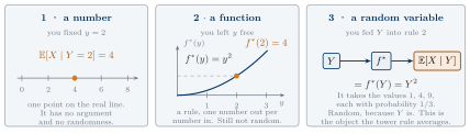
The three panels show the three objects. What they cannot show is the order, and the order is the content: each step changes what is fixed and what is free. The animation below puts that order back. Watch what is random at each moment, because for most of the scene the answer is nothing:
Randomness enters once, late, and it enters through the input. The function \(f^{*}\) was fixed by the joint density before anything was drawn, and it never changes. The closing frame carries \(\mathbb{E}[f^{*}(Y)] = 14/3\), which is the tower rule of Section 1.2 on this example.
Almost every confusion in the next three sessions is one of these three objects standing in for another. When you read \(\mathbb{E}[X \mid Y]\) somewhere, ask which panel of Figure 1 it is. If the expression sits inside an outer expectation, it is panel 3. If it is being differentiated with respect to its argument, it is panel 2. If it is equal to a specific number, it is panel 1.
The tower rule
Let \((X, Y)\) have joint density \(p(x, y)\) and let \(\mathbb{E}\Vert X \Vert < \infty\). Then \[ \mathbb{E}_{y \sim p}\Big[\,\mathbb{E}\big[X \mid Y\big]\,\Big] \;=\; \mathbb{E}_{x \sim p}\big[X\big] . \tag{4}\]
Proof.
Write the outer expectation as an integral against the marginal \(p(y)\), and substitute Equation 1: \[ \begin{aligned} \mathbb{E}_{y \sim p}\Big[\,\mathbb{E}\big[X \mid Y\big]\,\Big] &\;=\; \int \Big( \int x\, p(x \mid y)\, \mathrm{d}x \Big)\, p(y)\, \mathrm{d}y \\[2pt] &\;=\; \int\!\!\int x\, p(x \mid y)\, p(y)\, \mathrm{d}x\, \mathrm{d}y \\[2pt] &\;=\; \int\!\!\int x\, p(x, y)\, \mathrm{d}x\, \mathrm{d}y \;=\; \int x\, p(x)\, \mathrm{d}x \;=\; \mathbb{E}_{x \sim p}\big[X\big] . \end{aligned} \] The second line exchanges the order of integration. The third line uses \(p(x \mid y)\, p(y) = p(x, y)\), which is the definition of the conditional density, and then integrates \(y\) out. \(\;\blacksquare\)
The proof is three lines and one exchange of integration order. That exchange is the only place where an assumption is doing work, and Section 1.4 says which assumption.
The pull-out property
This is the second of the two results the Lemma needs, and it is the one that makes a cross term vanish.
Let \(g \colon \mathbb{R}^{d_y} \to \mathbb{R}\) be a function of \(y\) alone, and let \(X\) be scalar with \(\mathbb{E}|g(Y) X| < \infty\). Then \[ \mathbb{E}\big[\, g(Y)\, X \mid Y \,\big] \;=\; g(Y)\, \mathbb{E}\big[X \mid Y\big] . \tag{5}\]
Proof.
Fix a value \(y\). Inside the integral of Equation 1 the factor \(g(y)\) is a constant, so it comes out: \[ \begin{aligned} \mathbb{E}\big[g(Y) X \mid Y = y\big] &= \int g(y)\, x\, p(x \mid y)\, \mathrm{d}x = g(y) \int x\, p(x \mid y)\, \mathrm{d}x \\[2pt] &= g(y)\, \mathbb{E}\big[X \mid Y = y\big] . \end{aligned} \] That is an identity between two functions of \(y\). Evaluate both at \(Y\). \(\;\blacksquare\)
The sentence to remember is: once you condition on \(Y\), every function of \(Y\) behaves as a constant. Applied componentwise, Equation 5 gives the vector form the Lemma uses, \[ \mathbb{E}\big[\, \langle a(Y),\, Z \rangle \mid Y \,\big] \;=\; \big\langle a(Y),\, \mathbb{E}[Z \mid Y] \big\rangle , \tag{6}\] for any function \(a\) of \(y\) and any random vector \(Z\) with \(\mathbb{E}\Vert Z\Vert < \infty\): expand the inner product as a sum \(\sum_i a_i(Y) Z_i\), apply Equation 5 to each term, and use linearity.
Conditional expectation is linear in the conditioned variable: for constants \(a, b\) and random vectors \(X, Z\), \(\mathbb{E}[aX + bZ \mid Y] = a\,\mathbb{E}[X \mid Y] + b\,\mathbb{E}[Z \mid Y]\). The proof is the linearity of the integral in Equation 1, applied at each fixed \(y\). The Lemma uses this without comment.
What a measure-theoretic treatment would repair
Three steps above are honest only under assumptions this page does not verify. They are listed here once, and never mentioned again.
- The exchange of integration order in the tower-rule proof is Fubini’s theorem. It needs \(\mathbb{E}\Vert X\Vert < \infty\), which the statement assumes.
- Conditioning on \(p(y) = 0\). Equation 1 is undefined where the marginal vanishes. The general theory defines \(\mathbb{E}[X \mid Y]\) up to sets of probability zero, which is enough, because every statement below is an equality of expectations.
- Existence of the joint density. The general theory needs no density at all.
Every distribution in this course is a Gaussian, a mixture of Gaussians, an empirical distribution of data, or a smooth transformation of one of those. None of the three caveats ever bites.
- Section 2, in ten lines: the tower rule and Equation 6 are the whole proof of the projection Lemma.
- U3.T1 builds a marginal object by averaging conditional ones, which is Equation 4 with the conditioning variable renamed.
- Figure 1 is the reading aid for every conditional expectation in U3.
§2 — The projection Lemma
Here is the question. You observe \(Y\), and you want to guess \(X\). You must commit to a rule: a function \(f\) that turns each observed value into a guess. You will be scored by the mean squared error of your guess. Which \(f\) should you choose?
The answer is short, and it is the reason this session exists.
The space the question lives in
For a random vector \(Z\) in \(\mathbb{R}^{d}\) with \(\mathbb{E}\Vert Z\Vert^{2} < \infty\), write \[ \Vert Z \Vert_{L^{2}} \;=\; \big(\, \mathbb{E}\Vert Z\Vert^{2} \,\big)^{1/2} . \tag{7}\]
Equation 7 is a genuine distance between random vectors, and that is the point of introducing it: it makes the result below a statement about a right triangle, and lets you add lengths the way you learned to in school. Write \[ \mathcal{F}_Y \;=\; \Big\{\, f(Y) \;:\; f \text{ measurable},\; \mathbb{E}\Vert f(Y)\Vert^{2} < \infty \,\Big\} , \tag{8}\] the set of all square-integrable functions of \(Y\). The word measurable in Equation 8 rules out a class of pathological functions that nobody writes down on purpose; if you have not met the term, read it as “any function you could actually define”. Every rule you could commit to is a member of \(\mathcal{F}_Y\). The target \(X\) is generally not a member, because \(X\) is not a function of \(Y\) — if it were, you would not be guessing.
The Lemma
Let \((X, Y)\) be jointly distributed with \(\mathbb{E}\Vert X\Vert^{2} < \infty\), and set \(f^{*}(y) = \mathbb{E}[X \mid Y = y]\). Then:
(i) Pythagoras. For every \(f(Y) \in \mathcal{F}_Y\), \[ \mathbb{E}\big\Vert f(Y) - X \big\Vert^{2} \;=\; \mathbb{E}\big\Vert f^{*}(Y) - X \big\Vert^{2} \;+\; \mathbb{E}\big\Vert f(Y) - f^{*}(Y) \big\Vert^{2} . \tag{9}\]
(ii) Minimization. Consequently \(f^{*}\) minimizes \(\mathbb{E}\Vert f(Y) - X\Vert^{2}\) over all of \(\mathcal{F}_Y\), and it is the only minimizer, up to a set of \(Y\)-values of probability zero.
Claim (ii) reads straight off claim (i): the first term on the right of Equation 9 does not involve \(f\), and the second is non-negative and equals zero exactly when \(f(Y) = f^{*}(Y)\) with probability one. So the whole content is Equation 9, and Equation 9 is one expansion and one vanishing cross term.
Proof.
Step 0 — the terms are finite. First, \(f^{*}(Y) \in \mathcal{F}_Y\). For any component \(i\), conditional variance is non-negative, so \(\big(\mathbb{E}[X_i \mid Y]\big)^{2} \le \mathbb{E}[X_i^{2} \mid Y]\). Summing over \(i\) and taking expectations, the tower rule gives \(\mathbb{E}\Vert f^{*}(Y)\Vert^{2} \le \mathbb{E}\Vert X\Vert^{2} < \infty\). Every expectation below is then finite by the Cauchy–Schwarz inequality.
Step 1 — add and subtract. Insert \(f^{*}(Y)\) inside the norm and expand: \[ \begin{aligned} \mathbb{E}\big\Vert f(Y) - X \big\Vert^{2} &\;=\; \mathbb{E}\big\Vert \big(f(Y) - f^{*}(Y)\big) + \big(f^{*}(Y) - X\big) \big\Vert^{2} \\[2pt] &\;=\; \mathbb{E}\big\Vert f(Y) - f^{*}(Y) \big\Vert^{2} \;+\; \mathbb{E}\big\Vert f^{*}(Y) - X \big\Vert^{2} \;+\; 2\, C , \\[6pt] \text{where}\quad C &\;=\; \mathbb{E}\big\langle\, f(Y) - f^{*}(Y),\; f^{*}(Y) - X \,\big\rangle . \end{aligned} \]
Step 2 — the cross term is zero. Write \(a(Y) = f(Y) - f^{*}(Y)\), which is a function of \(Y\). Apply the tower rule to \(C\), then Equation 6, then Equation 3: \[ \begin{aligned} C &\;=\; \mathbb{E}\Big[\, \mathbb{E}\big[\, \langle a(Y),\, f^{*}(Y) - X \rangle \mid Y \,\big] \,\Big] && \text{(tower rule)} \\[2pt] &\;=\; \mathbb{E}\Big[\, \big\langle a(Y),\; \mathbb{E}\big[\, f^{*}(Y) - X \mid Y \,\big] \big\rangle \,\Big] && \text{(pull-out)} \\[2pt] &\;=\; \mathbb{E}\Big[\, \big\langle a(Y),\; f^{*}(Y) - \mathbb{E}[X \mid Y] \big\rangle \,\Big] && \text{(pull-out again, on } f^{*}(Y)\text{)} \\[2pt] &\;=\; \mathbb{E}\Big[\, \big\langle a(Y),\; 0 \big\rangle \,\Big] \;=\; 0 . && \text{(definition of } f^{*}) \end{aligned} \] The third line uses the pull-out property once more: \(f^{*}(Y)\) is itself a function of \(Y\), so conditioning on \(Y\) leaves it alone. The last line is Equation 3, which says \(\mathbb{E}[X \mid Y]\) is \(f^{*}(Y)\).
Step 3 — read off both claims. With \(C = 0\), step 1 is exactly Equation 9, which is claim (i). Claim (ii) follows as noted above. \(\;\blacksquare\)
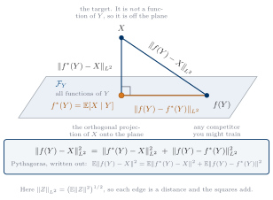
Figure 2 draws one competitor \(f(Y)\). The Lemma is a statement about every one of them, and what it asserts is an invariance: as \(f(Y)\) moves anywhere in the plane, the angle at \(f^{*}(Y)\) stays right and the vertical edge does not change length. An invariance under motion is not something a still can carry, so the animation below moves \(f(Y)\) along a closed loop and measures all three edges as it goes:
Two things in it are worth naming. The loop passes through \(f(Y) = f^{*}(Y)\), and there the horizontal edge collapses to zero while the hypotenuse falls to exactly the vertical edge — that is the minimizer, and it is the only place the error is the floor and nothing else.
And the three bars are measured, not drawn. They are \(L^{2}\) norms computed by Monte Carlo on the pair of PS1.2 below (\(X \sim \mathcal{N}(0,1)\), \(Y = X + 0.7\,\varepsilon\), \(n = 400\,000\)), and the scene is only allowed to render if the empirical cross term stays inside four standard errors of zero at every one of the \(241\) loop positions. It stays inside \(0.71\). A deliberately wrong projection, put through the identical test, reaches \(65\) — which is what makes the first number worth reporting.
Read Figure 2 as linear algebra. \(\mathcal{F}_Y\) is a linear subspace: sums and scalar multiples of functions of \(Y\) are functions of \(Y\). The inner product \(\langle Z, W \rangle_{L^{2}} = \mathbb{E}\langle Z, W\rangle\) makes it an inner-product space, and \(\Vert \cdot \Vert_{L^{2}}\) of Equation 7 is its norm. Step 2 says that the error of \(f^{*}\) is orthogonal to every element of the subspace. That is the defining property of an orthogonal projection, and Pythagoras is what orthogonal projections always give you.
The corollary that gets used
The Lemma is the theorem. The corollary below is the form three later sessions actually apply, and it is worth stating separately for that reason alone.
Fix a parametric family \(\{f_\theta\}\) — in practice a neural network with parameters \(\theta\) — with \(f_\theta(Y) \in \mathcal{F}_Y\) for every \(\theta\).
(a) Constant offset. The two objectives \[ \begin{aligned} \mathcal{L}_{\mathrm{target}}(\theta) &= \mathbb{E}_{(x, y) \sim p}\big\Vert f_\theta(y) - x \big\Vert^{2} , \\[2pt] \mathcal{L}_{\mathrm{proj}}(\theta) &= \mathbb{E}_{y \sim p}\big\Vert f_\theta(y) - f^{*}(y) \big\Vert^{2} , \end{aligned} \] differ by a constant that does not depend on \(\theta\). Hence they have the same minimizers and, wherever the gradients exist, the identical gradients \(\nabla_\theta \mathcal{L}_{\mathrm{target}} = \nabla_\theta \mathcal{L}_{\mathrm{proj}}\).
(b) Surrogate target. Let \(Z\) be any random vector with \(\mathbb{E}\Vert Z\Vert^{2} < \infty\) and \[ \mathbb{E}\big[Z \mid Y\big] \;=\; \mathbb{E}\big[X \mid Y\big] . \tag{10}\] Then \(\mathcal{L}_{\mathrm{target}}(\theta)\) and \(\mathbb{E}_{(z, y)}\Vert f_\theta(y) - z\Vert^{2}\) also differ by a constant that does not depend on \(\theta\) — same minimizers, same gradients.
Proof.
(a) is Equation 9 read with \(f = f_\theta\): the term \(\mathbb{E}\Vert f^{*}(Y) - X\Vert^{2}\) contains no \(\theta\).
(b) Apply Equation 9 twice. Once with the target \(X\), and once with the target \(Z\) — which is legitimate, because Equation 10 says the two targets have the same projection \(f^{*}\): \[ \begin{aligned} \mathbb{E}\big\Vert f_\theta(Y) - X \big\Vert^{2} &\;=\; \mathbb{E}\big\Vert f^{*}(Y) - X \big\Vert^{2} + \mathcal{L}_{\mathrm{proj}}(\theta) , \\ \mathbb{E}\big\Vert f_\theta(Y) - Z \big\Vert^{2} &\;=\; \mathbb{E}\big\Vert f^{*}(Y) - Z \big\Vert^{2} + \mathcal{L}_{\mathrm{proj}}(\theta) . \end{aligned} \] Subtract. The \(\theta\)-dependent term cancels, and what is left, \(\mathbb{E}\Vert f^{*}(Y) - X\Vert^{2} - \mathbb{E}\Vert f^{*}(Y) - Z\Vert^{2}\), has no \(\theta\) in it. \(\;\blacksquare\)
Same conditional mean.
Part (b) says you may throw away the regression target you cannot compute, and regress against any surrogate that has the same conditional mean. The two losses take different values. The minimizer is the same, and every gradient step is the same. Three sentences of proof, and it is the engine of half this course.
What \(X\), \(Y\) and \(Z\) will be
Nothing yet. That is deliberate.
The Lemma is a statement about two jointly distributed random vectors and a square loss. It is true whatever they stand for, and the later sessions supply three completely different substitutions. Learn it in this abstract form. If you attach it to one interpretation now, you will not recognize the other two when they arrive.
The next section is a slide, and the slide answers exactly this question.
§3 — The announcement
This section is one slide. It is reproduced in the notes because it is shown again, twice, in later sessions.
This Lemma will be used exactly three times.
- U3.T1 — to define the marginal velocity field: it is a conditional expectation of conditional velocities.
- U3.T2 — to prove the CFM theorem: swapping the unknown marginal target for a conditional surrogate leaves \(\theta\)-gradients unchanged (corollary (b)).
- U3.T2, detour D2 — to derive denoising score matching: same three lines, different random variables.
Tattoo it somewhere.
You are not supposed to understand items 1 to 3 yet. Every technical term in them belongs to a session that has not happened. You are supposed to recognize them when they arrive, and to know, when they do, that the argument is one you already have.
That is the whole purpose of announcing them now. A result you meet three times as a surprise is three separate difficulties. The same result, announced once and then recognized, is one.
§4 — Pushforwards, and what a generative model is
Reference for this section: (Murphy 2023) ch. 5, which covers the divergence and states the equivalence of Section 4.3 in its own notation; and (Lipman et al. 2024) §3.3, which is where the symbol \(\psi_{\#}\) of Section 4.1 comes from. Read that section with one caveat: the Guide states the push-forward for diffeomorphisms, so that it can also give the density formula. Equation 11 below states it for any measurable map, which is weaker and is all this session needs.
The rest of the session builds the second thing you need, which is the vocabulary to say precisely what the course is trying to do.
Pushforward
Let \(p\) be a distribution on \(\mathbb{R}^{d}\) and let \(\psi \colon \mathbb{R}^{d} \to \mathbb{R}^{d}\) be measurable. The pushforward \(\psi_{\#}\, p\) is the distribution of \(\psi(x)\) when \(x \sim p\). Equivalently, it is the unique distribution for which \[ \mathbb{E}_{y \sim \psi_{\#} p}\big[\, g(y) \,\big] \;=\; \mathbb{E}_{x \sim p}\big[\, g(\psi(x)) \,\big] \tag{11}\] holds for every bounded measurable \(g\).
Read Equation 11 as an instruction rather than as an equation: to sample from \(\psi_{\#}\, p\), sample from \(p\) and apply \(\psi\). That is the entire content, and the notation \(\psi_{\#}\) is fixed for the course.
You have already built one. UP.A §4.2 wrote \(x = \mu + \sigma\varepsilon\) with \(\varepsilon \sim \mathcal{N}(0,1)\), and observed that sampling is pushing a fixed noise source through a deterministic map. In the notation of Equation 11 that reparameterization is \(\mathcal{N}(\mu, \sigma^{2}) = \psi_{\#}\, \mathcal{N}(0, 1)\) with \(\psi(\varepsilon) = \mu + \sigma\varepsilon\). It was the first pushforward of the course, written before the word existed.
A generative model
\[ p_\theta \;=\; \big(\psi^{\theta}\big)_{\#}\, p_0 , \qquad p_0 = \mathcal{N}(0, I_d) . \tag{12}\]
Four elements, one sentence each.
- \(p_0 = \mathcal{N}(0, I_d)\) is the source. It is standard, it is fixed, and it is never learned. It costs nothing to sample from.
- \(\psi^{\theta}\) is the map, and it is the only learned object. Its parameters \(\theta\) are what a training run changes.
- \(p_\theta\) is the model: whatever distribution the map produces. You never write it down. You sample from it, by Equation 11.
- \(q\) is the data distribution, which you never write down either. You have samples \(x_1 \sim q\), and that is all you will ever have.
\(t\) runs over \([0, 1]\). \(t = 0\) is noise and \(t = 1\) is data. So \(p_0\) is the source, \(x_1 \sim q\) is a data point, and a map that generates runs from \(0\) to \(1\).
The literature on diffusion models runs the arrow the other way. This course translates all of it, and the translation lives in exactly one document, the Rosetta Stone. Outside that document the arrow never reverses.
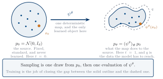
In this session \(\psi^{\theta}\) is one map, and how it is built is not the subject. U1 builds it as a composition of invertible layers. U2 builds it as the time-1 value of a differential equation. U3 changes what is learned altogether. The definition Equation 12 survives all three.
Maximum likelihood is a KL
You have samples from \(q\) and a family \(p_\theta\). The standard fit criterion is maximum likelihood. The following says it is also a divergence criterion, and being able to read it both ways is what makes the rest of the course possible.
Assume \(q\) has a density, that \(\mathbb{E}_{x_1 \sim q}\big[\log q(x_1)\big]\) is finite, and that \(p_\theta(x) > 0\) wherever \(q(x) > 0\). Then \[ \operatorname*{arg\,max}_{\theta}\; \mathbb{E}_{x_1 \sim q}\big[\, \log p_\theta(x_1) \,\big] \;=\; \operatorname*{arg\,min}_{\theta}\; \mathrm{KL}\big(q \,\Vert\, p_\theta\big) . \tag{13}\]
Proof.
Expand the divergence with the definition from UP.A §3.1 and split the logarithm: \[ \begin{aligned} \mathrm{KL}\big(q \,\Vert\, p_\theta\big) &= \mathbb{E}_{x_1 \sim q}\Big[\, \log \frac{q(x_1)}{p_\theta(x_1)} \,\Big] \\[2pt] &= \underbrace{\mathbb{E}_{x_1 \sim q}\big[\log q(x_1)\big]}_{\text{no } \theta} \;-\; \mathbb{E}_{x_1 \sim q}\big[\log p_\theta(x_1)\big] . \end{aligned} \] The first term is a property of the data alone — it has no \(\theta\) in it, and the assumption is exactly that it is finite. (Its negative is called the differential entropy of \(q\); the name is not used again.) So the two sides of Equation 13 differ by a constant, and minimizing one is maximizing the other. \(\;\blacksquare\)
The data sits in the first argument of the divergence. UP.A §3.3 showed what that costs: it is the mass-covering direction, the one that refuses to leave any part of \(q\) uncovered and pays by putting model mass where the data has none.
That is not a defect to be fixed here. It is a property of the objective, and it is one reason a model trained by maximum likelihood can produce samples that lie between the modes of the data. Notice it now; it returns whenever the course compares training criteria.
The problem this creates
Look at Equation 13 again, and read the quantity you have to compute: \(\log p_\theta(x_1)\), the log-density of the model at a data point.
You do not have that density. What you have is Equation 12, which is a recipe for sampling. Getting from a sampling recipe to a density value means undoing the map \(\psi^{\theta}\) at \(x_1\), and accounting for how much the map stretched or compressed volume on the way. Both halves are hard, and making them tractable is the technical content of the next two units.
That sentence is the bridge out of this session.
§6 — Problem set PS1.2
This is one of the two graded parts of PS1. The other, PS1.1, is the nine exercises embedded in the primer.
The setting upgrades the worked example of UP.A §2.6 from one dimension to \(d\), and then asks you to see the Lemma happen on a screen.
Let \[ X \sim \mathcal{N}(\mu_0, \sigma_0^{2} I_d) , \qquad Y = X + \sigma \varepsilon , \qquad \varepsilon \sim \mathcal{N}(0, I_d), \quad \varepsilon \perp X . \]
(a) Closed form. Compute \(\mathbb{E}[X \mid Y = y]\) explicitly, in terms of \(\mu_0\), \(\sigma_0\), \(\sigma\) and \(y\). Use the gaussian-algebra-toolkit sheet; the scalar case is item 9 on it, and the step from one dimension to \(d\) is one sentence, which you should write. State also \(\operatorname{Var}(X \mid Y = y)\), and say in one line what happens to your answer as \(\sigma \to 0\) and as \(\sigma \to \infty\).
(b) Numerical verification, \(d = 1\). Fix \(\mu_0 = 0\), \(\sigma_0 = 1\), \(\sigma = 0.5\). Draw at least \(20{,}000\) pairs \((y, x)\). Train a small multilayer perceptron \(f_\theta \colon \mathbb{R} \to \mathbb{R}\) with the square loss \(\mathcal{L}(\theta) = \mathbb{E}_{(x, y)}\Vert f_\theta(y) - x\Vert^{2}\). Plot the trained \(f_\theta\) against the closed form of part (a) on the same axes, over a range of \(y\) that the samples actually cover. Report the largest gap between the two curves on that range.
(c) The surrogate, empirically. Keep everything from (b), and replace the regression target \(X\) by \[ Z = X + \eta , \qquad \eta \sim \mathcal{N}(0, \tau^{2}), \quad \eta \perp (X, Y), \qquad \tau = 1 . \] First verify on paper, in one line, that \(\mathbb{E}[Z \mid Y] = \mathbb{E}[X \mid Y]\), which is Equation 10. Then retrain from the same initialization and the same seed, and produce two numbers and one plot:
- the two final loss values, which must differ;
- the largest gap between the two learned functions, which must not;
- one figure with the closed form of (a), the network of (b), and the network of (c) on the same axes.
Say in two sentences why the loss values differ, and by roughly how much you predicted they would before running it.
This exercise has a secret identity, to be revealed in U3.
You do not need any earlier session to do this. The network can be three Linear layers with Tanh between them and 64 hidden units; the optimizer can be Adam at \(10^{-3}\); a few thousand steps of full-batch or large-minibatch training is enough. The whole thing runs on a laptop CPU in under a minute.
Report your seed, and report it in your write-up. Two of the three numbers asked for in part (c) are only meaningful against a fixed seed.
Corollary (b) predicts that the two minimizers coincide, not that two training runs coincide. Your two learned functions will differ a little, from finite samples and finite optimization. The claim under test is that the gap between them is of the same size as the gap you would get by rerunning (b) twice with different seeds — and not of the size of the gap between either of them and, say, the constant zero function. Run that control if your numbers surprise you.
Where this session reappears
| From this session | Reappears in |
|---|---|
| The projection Lemma, Equation 9 | U3.T1 (to define an object); U3.T2 (to prove a theorem) |
| Corollary (b), “same conditional mean” | U3.T2, twice — the main line and detour D2 |
| The tower rule, Equation 4 | inside every application of the Lemma |
| Pushforward notation \(\psi_{\#}\) | U1.T1; U2.T1; U3.T1 |
| \(p_\theta = (\psi^{\theta})_{\#} p_0\), Equation 12 | U1.T1 (built by layers); U2.T1 (built by an ODE) |
| Maximum likelihood is a KL, Equation 13 | U1.T1 (the training objective); U2.T2 |
| The time arrow \(t = 0\) noise, \(t = 1\) data | everything from U3 on, without exception |
Next session
The next session opens U1 and takes the first of the three strategies of Section 5: make \(\psi^{\theta}\) invertible by construction, and read its volume change off the architecture. The result that makes it work is the change-of-variables theorem, and proving it in \(d\) dimensions is part of PS1.
Before then: PS1.1 is the primer’s nine exercises, and PS1.2 is Section 6. Both are due together.