UP.T1 — The Lemma of the Course

Flow-Based Generative Models · UFRJ · 2026.2

01Why this session exists

Where this course is going

• Discrete flows. Build the map out of invertible layers. Exact likelihood, restricted map.
• Continuous time. Let the map be the solution of a differential equation. The restriction goes; training now runs a solver inside every step.
• Flow Matching. Stop asking for the likelihood. Regress against a target you can write down.

Today is none of those. Today is the foundation all three stand on.

Eight minutes for the whole of block A. Do not explain any of the three phrases — they are place-markers, not content. If a hand goes up asking what a velocity field is, the answer is “U3.T1” and move on. The point of the slide is that the audience can locate today on a map.

The promise made today

We prove one result. Then we announce, on one slide, the three later sessions that use it.

When each of those three moments arrives, I will point back at this board.

Everything else in this session exists so that the promise can be stated precisely.

Say the joint-audience sentence out loud here: PGMAT has had the bootcamp, PESC has the self-study packet, and this session is where the two populations merge. It depends on UP.A and on nothing else — say that explicitly, because half the room is wondering whether they are behind.

Then state the two house rules: the Lemma is cited by name for the rest of the course, and every expectation in every loss carries its sampling subscripts. Point at the primer §5 drill as the contract.

02Conditional expectation, done properly

Three objects share one notation

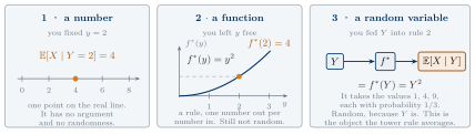
Ask it of every conditional expectation you meet: which panel is this?

Board work, 8 to 25 minutes. Draw the three-object diagram before showing this slide, on the running example \(Y \sim \mathrm{Unif}\{1,2,3\}\), \(X \mid Y = k \sim \mathcal{N}(k^2, 1)\) — it is the primer’s own example, so it costs nothing to set up.

Then, on the board and in full:

1. the tower rule, proved by Fubini in three lines. One honest sentence on the measure-theoretic caveats, and then never again.
2. the pull-out property, one line: once you condition on Y, every function of Y is a constant.

Leave both on a SIDE board. They are the entire proof of the next block, and the room should be able to look up at them while that proof runs.

The three objects, separated in time

The previous slide shows the three objects side by side. Side by side is the wrong relation: they are not three alternatives, they are one object being BUILT, and each step changes what is fixed and what is free. This scene puts that order back.

Four moments to name as they pass:

1. y is fixed. The dot is a NUMBER.
2. y ranges. The dot traces a curve, and the curve is a FUNCTION — still nothing random anywhere on the screen.
3. Only now does Y become random, and it is the INPUT that becomes random.
4. The die settles six times, and the image lands on 1, 4 or 9. That is the RANDOM VARIABLE.

The closing frame carries E[f*(Y)] = 14/3, which is the tower rule on this example — the side board is where they should look while it appears.

03The projection Lemma

The statement

Write \(f^{*}(y) = \mathbb{E}[X \mid Y = y]\).

Then for every square-integrable function \(f\) of \(Y\): \[ \mathbb{E}\big\Vert f(Y) - X \big\Vert^{2} = \mathbb{E}\big\Vert f^{*}(Y) - X \big\Vert^{2} + \mathbb{E}\big\Vert f(Y) - f^{*}(Y) \big\Vert^{2} . \] So \(f^{*}\) minimizes the left side, and it is the only minimizer.

Square-integrable, throughout: \(\mathbb{E}\Vert X\Vert^{2} < \infty\) and \(\mathbb{E}\Vert f(Y)\Vert^{2} < \infty\).

The proof is on the board. It is one expansion, and one cross term that dies.

25 to 50 minutes, all board, no gaps. This is the one proof of the day that gets none.

Order: add and subtract f(Y) inside the norm; expand into three terms; kill the cross term by tower rule then pull-out then the definition of f; read off BOTH claims at once.

Draw the right triangle. X above the plane, f*(Y) its foot, f(Y) a third vertex in the plane. Say the words “orthogonal projection” and leave the picture up.

Then the corollary, three lines, deliberately anticlimactic: (a) the two objectives differ by a constant free of \(\theta\), so identical gradients; (b) any surrogate Z with E[Z|Y] = E[X|Y] gives the same minimizer and the same gradients. Say the phrase “same conditional mean” and make them repeat it.

Do NOT say what X, Y, Z will be. The abstraction is the product.

What the picture says

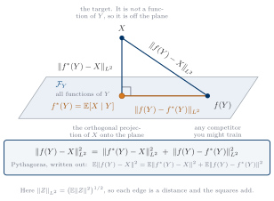
The vertical edge is a floor. The horizontal edge is the only part training can move.

Use this slide only if the board triangle came out badly, or as the thing left on screen while the corollary is proved. Here \(\Vert Z\Vert_{L^2} = (\mathbb{E}\Vert Z\Vert^2)^{1/2}\), so the edges are distances and the squares add.

The angle that never opens

The previous slide is one competitor. The Lemma is about all of them, and its visual content is an invariance: f(Y) goes anywhere it likes in the plane, and the right angle does not open. Point at the blue bar and say “watch that one” — it does not move once.

Two moments worth stopping on:

• The pause where f(Y) = f*(Y). The orange bar reads 0.0000 and the hypotenuse reads 0.5731, equal to the blue bar. That is the minimizer, and it is the one place the error is only the floor.
• The closing frame. The bars are MEASURED, not drawn: L2 norms by Monte Carlo on the PS1.2 pair, and the cross term stays inside 0.71 standard errors of zero across all 241 positions. A deliberately wrong projection reaches 65, which is what makes the first number mean something.

Say that last part out loud. It is the difference between a picture that illustrates a theorem and a picture that was checked against one.

04The announcement

This Lemma will be used exactly three times

1. U3.T1 — to define the marginal velocity field: it is a conditional expectation of conditional velocities.
2. U3.T2 — to prove the CFM theorem: swapping the unknown marginal target for a conditional surrogate leaves \(\theta\)-gradients unchanged (corollary (b)).
3. U3.T2, detour D2 — to derive denoising score matching: same three lines, different random variables.

Tattoo it somewhere.

PROTECTED SLIDE. It is a named, versioned artifact, and it is shown again — grayed out, with the current use highlighted — in U3.T1 and in U3.T2. Do not edit the wording without editing those two sessions.

Eight minutes, and they are not filler. Read the three items SLOWLY.

Then say the thing that makes the device work: “you are not supposed to understand items 1 to 3 yet. You are supposed to recognize them when they arrive.” Say it in those words. A promise that is not announced as a promise is just a confusing slide.

If the session is running late, this is the block that does NOT get compressed. Compress block E instead.

05Pushforwards, and what a model is

Pushforward

\(\psi_{\#}\, p\) is the distribution of \(\psi(x)\) when \(x \sim p\): \[ \mathbb{E}_{y \sim \psi_{\#} p}\big[ g(y) \big] = \mathbb{E}_{x \sim p}\big[ g(\psi(x)) \big] \quad \text{for every bounded } g . \]

Read it as an instruction: to sample from \(\psi_{\#}\, p\), sample from \(p\) and apply \(\psi\).

You built one in the primer: \(x = \mu + \sigma\varepsilon\) is \(\mathcal{N}(\mu, \sigma^2) = \psi_{\#}\,\mathcal{N}(0,1)\).

The symbol \(\psi_{\#}\) is the course standard, after (Lipman et al. 2024) §3.3.

The reparameterization callback is worth ten seconds of pause. They wrote the first pushforward of the course before the word existed, and they wrote it as a trick for getting gradients through a sampler.

A generative model is a pushforward of noise

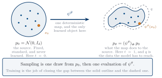
\[ p_\theta = \big(\psi^{\theta}\big)_{\#}\, p_0 , \qquad p_0 = \mathcal{N}(0, I_d) \]

One sentence per element, and no more. The source is fixed and never learned. The map is the only learned object. The model is what the map does to the source — you never write it down, you sample from it. And q is the data, of which you have samples and nothing else.

Then state the time convention of the course, out loud, for the first time in a live session: t runs over [0,1], t = 0 is noise, t = 1 is data. Say that the diffusion literature runs it the other way and that the translation lives in exactly one document. Then never revisit it.

Maximum likelihood is a KL

\[ \operatorname*{arg\,max}_{\theta}\; \mathbb{E}_{x_1 \sim q}\big[ \log p_\theta(x_1) \big] \;=\; \operatorname*{arg\,min}_{\theta}\; \mathrm{KL}\big(q \,\Vert\, p_\theta\big) . \]

Two lines: expand the divergence, drop the term with no \(\theta\) in it.

The data sits in the first argument — the mass-covering direction of the primer’s §3.3.

But maximum likelihood needs \(\log p_\theta(x_1)\), and the definition above only gives you samples.

58 to 75 minutes. Prove it live; it really is two lines. If the clock is against you, sketch it and say “the details are two lines, and they are in the notes” — this is the block the L3 designates as compressible, precisely because the notes carry it in full.

The closing sentence is the bridge out of the session. Getting a density value out of a sampling recipe means undoing the map and accounting for the volume it moved. Both halves are hard. That is U1 and U2.

06What comes next

Why likelihoods will be hard

Unit	Strategy	What it costs
U1	invertible by construction	what the map is allowed to be
U2	volume change by calculus	a solver inside every training step
U3	refuse to play	nothing yet — this is where the Lemma returns

And one thing that cannot even be written down yet: comparing two whole paths of distributions, rather than two distributions.

Three phrases, no formulas, and this is the block that absorbs any overrun. If there is no time, say the U3 row alone and go to PS1.2.

“Path” here is a word, not a definition. Do not draw one.

PS1.2 — the Lemma, in closed form and on a machine

\(X \sim \mathcal{N}(\mu_0, \sigma_0^{2} I_d)\), and \(Y = X + \sigma\varepsilon\).

(a) Compute \(\mathbb{E}[X \mid Y = y]\) in closed form, from the toolkit sheet.

(b) In \(d = 1\): train a small network on samples \((y, x)\) with the square loss. Plot it against your closed form.

(c) Replace the target \(X\) by \(Z = X + \eta\) with \(\mathbb{E}[\eta \mid Y] = 0\). Retrain. The losses differ; the learned function does not.

This exercise has a secret identity, to be revealed in U3.

Two minutes. Part (c) is the corollary, made visible: the room should leave expecting the two curves to land on top of each other, and mildly annoyed that the loss values do not match.

Say clearly that nothing here needs the bootcamp — three Linear layers, Tanh, Adam, one minute on a CPU. The notes carry that contract in a box, so PESC students are not left guessing.

Do NOT say what the secret identity is. The reveal is scheduled in U3.T2, detour D2, and the solution key must not leak it either.

References

Lipman, Yaron, Marton Havasi, Peter Holderrieth, Neta Shaul, Matt Le, Brian Karrer, Ricky T. Q. Chen, David Lopez-Paz, Heli Ben-Hamu, and Itai Gat. 2024. “Flow Matching Guide and Code.” https://arxiv.org/abs/2412.06264.