U0.L5 — Solvers by Hand and a JAX Crash Course

Session U0.L5 · date: see calendar-map

Slides Slides PDF

This session closes the bootcamp, and it builds two things.

The first is common/odesolve.py: Euler, Heun, RK4 and one adaptive method, written from scratch, each one reporting what it cost. The previous theory session (U0.T5) derived all four on paper. Today they become code, and the code is not a demonstration — U3.L1 imports this file to draw the first samples of the course’s first Flow Matching model. The pictures of your first generative model will be drawn by the solver you write today.

The second is a JAX primer. Three later sessions have a JAX moment in them (U1.L1, U2.L1, U3.L1), and a language switch in the middle of a hard topic is expensive. So the switch happens here, on a problem you already understand completely, where the only new thing is the language.

Why JAX at all, stated plainly, because the choice deserves an argument and not a fashion. Three reasons. First, grad, vmap and jit make several of this course’s constructions clearer than their PyTorch equivalents — the per-sample Jacobians behind a coupling layer’s log-determinant in U1.L1 are the standard example. Second, diffrax is the strongest differential-equation library in the ecosystem, and U2.L1 uses it as a professional mirror of the module you write today. Third, a large part of this literature is now published as JAX code, and you must be able to read it. PyTorch remains this course’s primary language. The JAX moments are always mirrors, never the only path.

Format. A module and two notebooks. common/odesolve.py joins train.py, unet.py and eval.py in the package you have been building since U0.L1. lab-u0l5.ipynb drives the solver work; jax-primer.ipynb is the primer, and it stands alone.

Everything here runs on CPU, and that is a hard requirement rather than a convenience. These notes and both notebooks are the core of the self-study packet that PESC students receive at enrollment, and a packet reader has arbitrary hardware. Nothing on this page needs a GPU.

Every number in these notes was measured. The runs behind the figures are in scripts/python/fig_u0_l5_solvers.py, seeded, and the values are recorded in scripts/python/_outputs/u0l5_solvers.json. The one exception is the wall-clock timing of Section 5, and Section 5.3 says exactly in what sense it is an exception.

Standing reference for the differential-equation material and for diffrax: Kidger (Kidger 2022).

A · The two builds, and who consumes them

Reused in: U3.L1, U1.L1, U2.L1, and the PESC packet.

Every session of this bootcamp was justified by its reappearance later. Here are today’s two, with their consumers named.

Table 1: The two builds of this session.

Artifact	Where it lives	Who imports it
ode-solvers-scratch	common/odesolve.py	U3.L1 (ODE sampling); the PESC packet
jax-primer	labs/jax-primer.ipynb	the JAX moments of U1.L1, U2.L1, U3.L1; the PESC packet

There is a second audience for both, and it changes how they are written. Some of the people who read your notebook will be PESC students who were not in the room, who have no lecturer to ask, and who meet this course through the packet. So the notebooks carry full prose between the cells, every TODO is followed by a check that either passes or explains itself, and the solutions ship with the packet rather than a week later.

That is not bureaucracy. It is the ordinary standard for onboarding material, and you are writing onboarding material for colleagues you have not met.

B · The solver module

The contract comes first, and it is frozen

U0.L4 froze two interfaces before writing any code, for the reason that four later sessions import them from a written specification rather than from whatever the code happens to do. The same discipline applies here.

common/odesolve.py

odeint(f, x0, t0, t1, method="rk4", n_steps=None,
       rtol=None, atol=None, return_traj=False)
    -> x1                   # a SolverOutput: a Tensor carrying .nfe
    -> (ts, xs)             # if return_traj=True; xs carries .nfe

METHODS = ("euler", "heun", "rk4", "adaptive_heun")

1. f(t, x) — time first. t is a scalar tensor, x has the shape of x0.
2. x0 has shape (B, d). The state is batched by construction.
3. Every call reports its NFE.

Each of the three laws is inherited, and each was decided somewhere earlier.

Law 1 is the U0.T5 convention, and its value is that it is also the convention of torchdiffeq and diffrax. A right-hand side you write against this signature is one the professional libraries accept unchanged, which is what makes U2.L1 a change of library rather than a rewrite. The two orderings are equally arbitrary in isolation; agreeing with the ecosystem is not.

Law 2 says the batch is not an afterthought. A generative model is sampled in batches, so the solver takes batches. Notice what this does not require: the step loop is an ordinary Python loop over steps, and the batch dimension is carried by the tensor operations inside it. There is no vmap in this file and none is needed. (Section 4.3 is about the case where you do need one, and it is a different case.)

Law 3 is the one worth arguing for, because it is the one people leave out. NFE — the number of evaluations of \(f\) — is this course’s cost currency. U2 watches it grow during training and it hurts; U3 is largely about making it small. A solver that hides its NFE cannot be compared with another solver, and a comparison you cannot make is a comparison you will not make.

How the cost travels with the answer

The frozen signature says odeint returns x1. It also says the NFE comes back. Those two are reconciled the same way common/eval.py reconciled the same tension in U0.L4: the returned value is the thing the contract promises, and it carries its own metadata.

class SolverOutput(torch.Tensor):
    nfe: int
    method: str
    n_steps: int
    accepted: int | None      # adaptive only
    rejected: int | None      # adaptive only

SolverOutput is a torch.Tensor. It prints, indexes, broadcasts and serializes like one, so every call site written against -> x1 works.

FIDValue did this for a float in U0.L4, so that an FID could not be compared across measurement protocols without the code objecting. The reasoning is identical here. A warning in a docstring does not survive contact with a results table. Making the cost travel with the number is what stops it from being forgotten at the exact moment it matters.

One honest limitation, worth knowing before it surprises you: the attributes do not survive arithmetic. (x1 - x0).nfe raises. Read .nfe from the value the solver returned.

The four TODOs

The four implementations are transcriptions. That is deliberate: U0.T5 derived every one of them, and a lab that re-derives what the theory session proved wastes the only 90 minutes in which the code gets written.

TODO 1 — Euler. One line of arithmetic, one evaluation per step.

\[ x_{n+1} \;=\; x_n + h \, f(t_n, x_n) . \]

TODO 2 — Heun. Predict with Euler, read the field at the provisional endpoint, average the two velocities. Two evaluations per step.

\[ \begin{aligned} k_1 &= f(t_n, x_n) , \\ k_2 &= f(t_n + h, \, x_n + h k_1) , \\ x_{n+1} &= x_n + \tfrac{h}{2}(k_1 + k_2) . \end{aligned} \]

TODO 3 — RK4. Four evaluations per step, weights \(\tfrac{1}{6}, \tfrac{2}{6}, \tfrac{2}{6}, \tfrac{1}{6}\). Transcribe the tableau from the U0.T5 notes — the tableau is the table of coefficients that defines a Runge–Kutta method, and this course is a consumer of tableaux rather than a designer of them. This TODO is mechanical on purpose — the interesting part of RK4 is not its arithmetic but its slope, and you measure that in Section 3.

TODO 4 — Adaptive Heun. The only one with a decision in it. Both the order-1 and the order-2 estimate come out of the same two evaluations, because \(k_1\) alone is the Euler step:

\[ \begin{aligned} \hat{x}_{n+1} &= x_n + h k_1 & &(\text{order } 1) , \\ x_{n+1} &= x_n + \tfrac{h}{2}(k_1 + k_2) & &(\text{order } 2) . \end{aligned} \]

Their difference estimates the local error. It is compared against the scale \(\mathrm{sc}_i = \texttt{atol} + \texttt{rtol} \cdot \max(|x_{n,i}|, |x_{n+1,i}|)\), component by component, and the step is accepted when the normalised error is at most 1. Accepted or rejected, the next step size comes from the same damped and clipped rule of U0.T5, with safety factor \(0.9\) and clips \(0.2\) and \(5\).

Two details of TODO 4 are easy to get wrong, and both are checked in the notebook.

Propagate the higher-order value. You computed it; keep it. The technique has a name — local extrapolation — and the alternative wastes the better of the two estimates you paid for.

Update the step size after a rejection too. A rejected step that retries at the same size rejects again, forever. The controller’s rule is unconditional.

The error estimate is a tensor of the shape of the state, and the controller needs one number. The module reduces it by a root-mean-square over every element of the batched state, which means one step size serves the hardest sample in the batch.

That is what torchdiffeq and diffrax do, and it is the honest choice rather than a shortcut: a per-sample step size would make NFE a per-sample quantity, and the batch would stop being a batch. It also means an outlier in the batch is paid for by everyone — which is a real cost of batched sampling, and one you will meet again in U2.

The checkpoint: your own version of the spiral

The first check reproduces Figure 1 — the icon of U0.T5 — with your Euler and your RK4.

Figure 1: Explicit Euler on the harmonic oscillator, step \(h = 2\pi/40\). (a) The phase plane over three periods: the exact orbit is the unit circle, RK4 stays on it, and Euler leaves it and ends at radius \(4.32\). (b) The energy against time. This is the figure of U0.T5, and the checkpoint asks you to make it yourself.

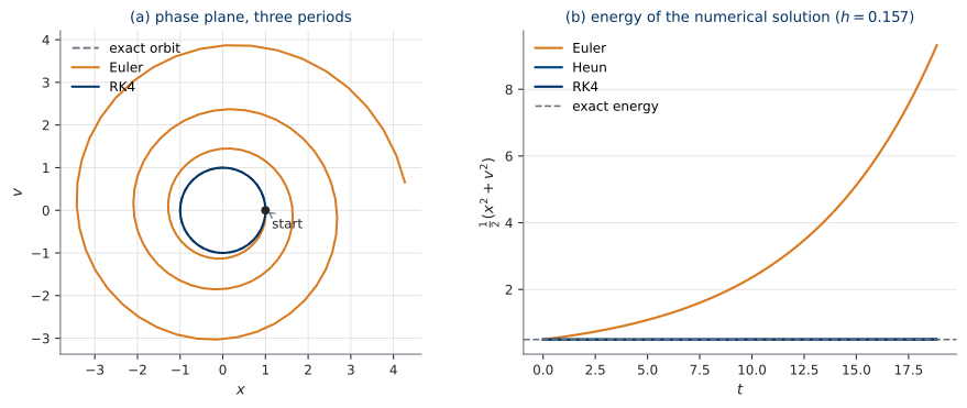
The check is not that the plot is pretty. Euler on this problem multiplies the energy by exactly \(1 + h^2\) per step, so the notebook asserts your solver’s energy ratio against that number. A hand-written solver that draws a plausible spiral with the wrong growth factor has a bug, and the assert finds it where the eye does not.

This module integrates forward. It does not differentiate through the integration, and it has no adjoint — that is U2.T1’s subject.

The scope is a teaching decision, not an oversight. Sampling is inference: no gradient is needed to draw a sample. Nothing in the file blocks autograd, since every operation is a plain torch operation, and a gradient will flow if you ask for one. What it will cost you in memory is precisely the problem U2.T1 exists to solve.

C · The convergence study

Collecting the prediction

Exercise 2 of U0.T5 asked you to predict the three slopes of a log-log plot of global error against step size, before making the plot. The answer was 1, 2 and 4, and the reasoning was that a global error of \(C h^p\) becomes a straight line of slope \(p\) under logarithms.

Now you make the plot with your own solvers, and the measured slopes are the check on your implementation. This is not a ritual. Measuring the order is the standard way to find a bug in a Runge–Kutta method, because a transcription error in the tableau usually leaves a method that still converges, still looks reasonable, and converges at the wrong rate. A hand-written RK4 that scores slope 3 has a typo, and the slope is what finds it.

The accounting table

The notebook prints the cost of each method at each step size. Reading it is the point of the block, so here is the row that matters, measured with the module of Section 2 on the harmonic oscillator over one period, at a matched budget of 4000 evaluations.

Table 2: The same cost, spent three ways. Every method here evaluated the field exactly 4000 times.

Method	Steps at NFE \(=4000\)	Global error at \(t = 2\pi\)
Euler	4000	\(4.9 \times 10^{-3}\)
Heun	2000	\(1.0 \times 10^{-5}\)
RK4	1000	\(8.2 \times 10^{-11}\)

Almost eight orders of magnitude separate the ends of Table 2 — a factor of \(6 \times 10^{7}\) — and nobody spent more than anybody else. That is the argument for high order stated as sharply as it can be stated, and it is why the notebook asks you to answer one question in writing: at an error budget of \(10^{-4}\), which row do you choose?

The answer has a caveat, and the caveat is the part that matters later. Table 2 assumes you want high accuracy. At a loose tolerance the three methods are much closer together, and at the extreme — one or two evaluations in total — a high-order method has no advantage at all, because it has not taken enough steps for its order to express itself. Sampling a generative model at 4 NFE lives in exactly that regime.

The tolerance sweep

The adaptive method does not take a step size. It takes a pair of tolerances, and it decides. So the study to run on it is a different one: sweep the request and watch what you get.

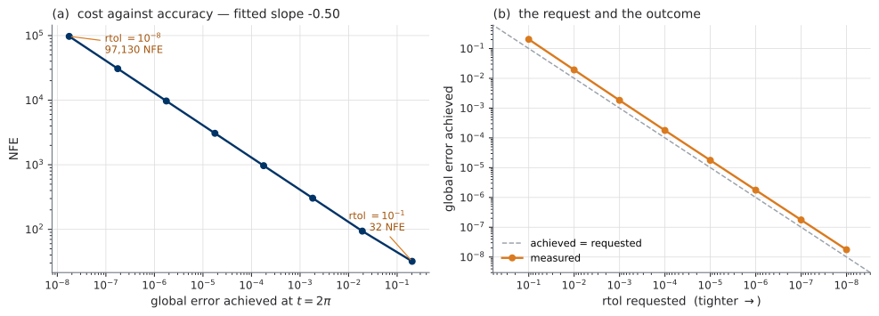
Figure 2: The adaptive Heun(2)/Euler(1) pair on the harmonic oscillator over one period, rtol swept from \(10^{-1}\) to \(10^{-8}\) with atol \(=\) rtol\(/100\) throughout. (a) NFE against the error actually achieved, log-log; the fitted slope is \(-0.50\). (b) The achieved error against the requested rtol, with the diagonal drawn: the outcome tracks the request across eight decades, at a fixed offset of about \(1.8\times\).

Three readings of Figure 2, and the notebook asks for all three.

The tolerance is a request, and it is honoured. Panel (b) is a straight line parallel to the diagonal. That is not guaranteed by anything — the controller bounds a local error estimate, and what panel (b) plots is the global error at the end. On this problem the two are proportional, which is the good case. On a badly conditioned problem they are not, which is why “I set rtol to \(10^{-6}\)” is a statement about what you asked for and never about what you got.

The cost of accuracy has a slope, and the slope is the order. The fitted slope of panel (a) is \(-0.50\), and \(-1/2\) is what an order-2 method predicts: to reduce the local error by a factor of \(10\) you shrink \(h\) by \(10^{1/2}\), and NFE goes as \(1/h\). Halving your error costs you \(\sqrt{2}\) times as much work with this method, and would cost \(2^{1/5}\) times as much with a fifth-order one. Section 5 measures exactly that difference.

Rejections are rare, and that is the controller working. Across all eight runs the solver rejected \(0, 0, 1, 1, 2, 3, 3\) and \(4\) steps respectively — out of up to 48 561 accepted. The safety factor of \(0.9\) is what buys that: it makes each proposed step slightly more conservative than the estimate suggests, so a marginal step is not immediately thrown away. A rejected step costs its evaluations and produces no progress, so a good controller rejects rarely and a controller that rejects constantly is misconfigured.

U0.T5 named two ways of getting the tolerances wrong. Figure 2 is where you can see both.

Too loose is the left end of panel (a): 32 evaluations, and an error of \(0.2\) on a trajectory whose whole radius is \(1\). The solver returned quickly, and it returned a smooth, plausible, entirely wrong orbit. Nothing complained. This is the dangerous failure, and the test for it is to halve both tolerances and re-run: if the answer moves by more than you can accept, the original answer was not converged.

Too tight is the right end: 97 130 evaluations, an error of \(1.8 \times 10^{-8}\), and a cost 3035 times the loose run. On a toy problem that is a few seconds. On a learned velocity field it is the difference between sampling in a minute and sampling over lunch, and the extra digits are far below the noise of everything else in the pipeline. This is the cheap failure — you notice it immediately, and it costs only time.

D · JAX in five moves

The primer has one organising sentence, and everything in it is an elaboration of that sentence.

JAX is NumPy, plus function transformations, plus explicit randomness.

Each of the three parts costs something. jnp is NumPy’s API over immutable arrays; the transformations require your functions to be pure; and explicit randomness means a random number generator is an argument you pass rather than a global you disturb. The rest of this section is what you get in exchange.

Scope, declared. The primer teaches five moves and stops. There is no flax and no optax beyond a single mention that they exist and appear in U3.L1’s JAX moment; there is nothing about sharding or TPUs. The primer optimizes for reading research JAX and for mirroring this course’s constructions. It does not optimize for writing production JAX, which is a different skill with a different book.

Move 1 — Pure functions and jnp

jnp is NumPy with immutable arrays. x[i] = v is an error; the replacement is a functional update that returns a new array.

y = x.at[i].set(v)        # returns a new array; x is unchanged

The price is real and it is worth stating once, honestly: you give up in-place mutation, and with it a family of comfortable patterns. What you buy is that a JAX function can be transformed — differentiated, vectorized, compiled, or all three — because a transformation needs to know that calling your function twice with the same arguments does the same thing twice. A function that reads a global counter, writes to a list, or prints, cannot be safely traced. Purity is the price of transformability, and the four moves below are what it purchases.

Move 2 — grad

jax.grad(f) returns a function: the gradient of f with respect to its first argument. f must return a scalar.

import jax, jax.numpy as jnp

def loss(theta, x):
    return jnp.sum((theta * x - 1.0) ** 2)

dloss = jax.grad(loss)            # a new function, same signature
g = dloss(theta, x)               # the gradient, same pytree as theta

There is no tape, no .backward(), and no .grad attribute on anything. The gradient is a function of the same shape as the original, and jax.value_and_grad gives you both outputs at the cost of one.

The check on it is one you have run twice already. U0.L1 introduced the finite-difference ritual and U0.L2 repeated it; here it is a third time, against jax.grad:

\[ \frac{\partial f}{\partial \theta_i} \;\approx\; \frac{f(\theta + \varepsilon e_i) - f(\theta - \varepsilon e_i)}{2\varepsilon} . \]

By now the ritual should be a reflex. It costs three lines, it takes a second, and it is the only thing that distinguishes a gradient from a plausible array of numbers.

Move 3 — vmap

jax.vmap maps a function over a batch axis without the function knowing about batches. You write the mathematics for one sample; vmap supplies the axis.

That is a convenience for a forward pass and something considerably more than a convenience for a gradient. The quantity below is genuinely awkward to obtain in eager PyTorch — eager meaning the ordinary mode in which each operation runs as the interpreter reaches it, rather than being recorded and compiled first — and the awkwardness is why people do not look at it:

per_sample = jax.vmap(jax.grad(loss_one), in_axes=(None, 0, 0))(params, xs, ys)

loss_one is the loss of a single sample and has no batch dimension anywhere in its body. jax.grad differentiates it. vmap runs the whole composition across the batch, and in_axes=(None, 0, 0) says the parameters are shared while the inputs and targets are mapped. The result is one gradient per sample.

Here is what that lets you see.

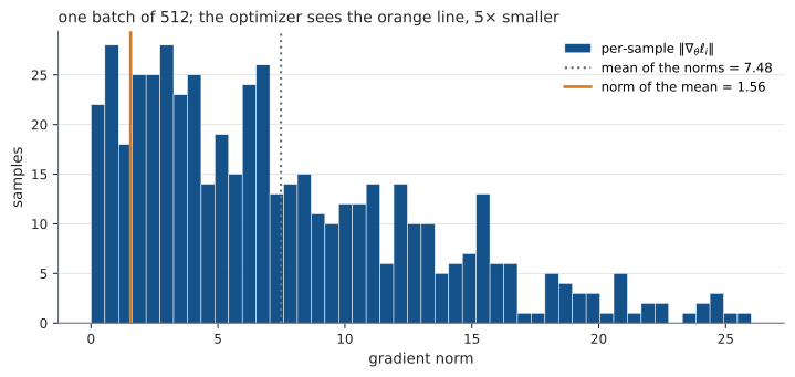
Figure 3: Per-sample gradient norms of a small MLP’s squared-error loss over one batch of 512, computed with vmap(grad(.)). The dotted line is the mean of the 512 norms, \(7.48\). The solid line is the norm of the mean gradient — the single vector the optimizer actually applies — at \(1.56\), smaller by a factor of \(4.8\). The distribution runs from \(0.003\) to \(26.0\).

The gap between the two lines in Figure 3 is cancellation: the per-sample gradients point in partly opposing directions, and the average is shorter than its parts. That is not a pathology, it is what averaging a batch is. But it means the number the optimizer sees is not a typical sample’s number, and the spread behind it — a factor of nearly \(10^4\) between the smallest and largest norm here — is invisible from the batch gradient alone.

Before the figure is believed, the notebook checks the machinery: vmap(grad(f)) on one sample against grad(f) on that sample, in a plain Python loop. The measured deviation is zero to machine precision — exactly \(0\) in the run behind this figure, and of order \(10^{-16}\) in the notebook’s own configuration. vmap is not an approximation of the loop; it is the same computation with a different execution order.

U1.L1 computes the log-determinant of a coupling layer’s Jacobian, per sample, with jax.jacfwd. That is this same composition with a different inner transformation, and this TODO is its warm-up.

Move 4 — jit

jax.jit(f) compiles f with XLA. The whole of the tracing model that you need fits in three sentences.

1. JAX runs your Python once, with abstract placeholder values, and records the operations. That recording is what gets compiled.
2. The recording is cached per input shape and dtype, so a new shape re-traces and re-compiles.
3. Because the trace sees placeholders rather than numbers, Python control flow that branches on a value cannot be recorded.

Point 3 is the classic trap, and the primer plants it rather than describing it:

@jax.jit
def f(x):
    if x > 0:          # TracerBoolConversionError
        return x
    return -x

Run the cell, read the error, then fix it with jnp.where. An error message you have met once is a different thing from an error message you have read about, and this is the error message every newcomer to JAX meets first.

Move 5 — Pytrees and PRNG keys

A pytree is any nest of containers with arrays at the leaves — a dict of dicts of arrays is the usual shape of a parameter set. Every JAX transformation accepts and returns pytrees, which is why jax.grad of a loss over a dict of parameters returns a dict of the same shape, and why jax.tree.map applies an update elementwise across the whole nest.

Randomness is the other half, and it is the part with a lesson in it for this course.

key = jax.random.key(0)
key, sub = jax.random.split(key)      # never reuse a key
x = jax.random.normal(sub, (batch, d))

There is no global seed and no hidden state. A random function takes a key and returns the same value for the same key, always. To get fresh randomness you split the key, and you use each key once.

This is stricter than what you did in U0.L2, and it is stricter in exactly the direction the hygiene stack was pushing. There, reproducibility was a discipline: seed the three generators, record the seed, remember not to call torch.randn in a place that changes the stream. Here it is not a discipline, because a key you forget to split is a bug you can see in the code, and a function’s randomness is visible in its signature.

JAX makes the seeding discipline structural. Randomness is an argument; reproducibility is the default.

E · The same ODE in diffrax

The adapter

diffrax wants f(t, y, args). You have f(t, x). The adapter is two lines, and writing it teaches the shape of the API:

def harmonic_jax(t, y, args):
    return jnp.array([y[1], -y[0]])

term = diffrax.ODETerm(harmonic_jax)
sol = diffrax.diffeqsolve(
    term, diffrax.Tsit5(), t0=0.0, t1=float(2 * jnp.pi), dt0=0.01, y0=y0,
    stepsize_controller=diffrax.PIDController(rtol=1e-6, atol=1e-8),
)

Every argument in that call is one you now understand. Tsit5 is a Runge–Kutta tableau of order 5 with an embedded estimate of order 4 — the same construction as your TODO 4, with better coefficients and more stages. PIDController is the step-size rule of Section 2 with a more careful smoothing law. dt0 is the first step, which the controller then overrides.

The cross-check

Two independent solvers, one problem. If they disagree, one of them is wrong, and finding out which is a far better use of ten minutes than trusting either.

The notebook runs diffrax’s Tsit5 at rtol \(=10^{-12}\) and your RK4 at 4000 fixed steps, and asserts their agreement. The measured difference is \(4.1 \times 10^{-13}\). Your solver and a professional library describe the same trajectory to within the arithmetic.

That is the good news. Here is the rest of it.

Figure 4: The adaptive Heun(2)/Euler(1) of Section 2 against diffrax’s Tsit5 on the same problem over the same tolerance sweep. Horizontal axis: the error actually achieved. Vertical axis: NFE. At the tightest accuracy the hand-written method reached — \(1.8 \times 10^{-8}\), for 97 130 evaluations — Tsit5 needs about 360.

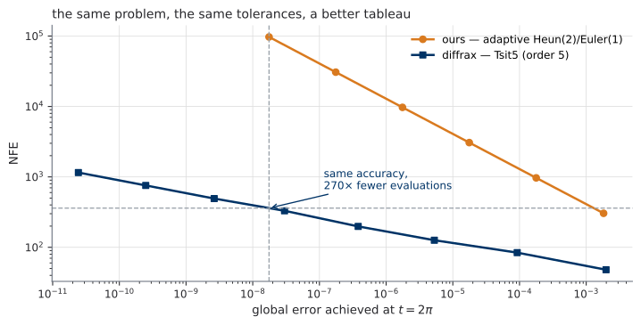
A factor of 270, at the same accuracy, on the same problem. The two lines in Figure 4 are not close and they are diverging, because their slopes differ: an order-5 method’s cost curve is much flatter than an order-2 method’s, and the tighter the tolerance the wider the gap.

Read the figure twice.

The first reading is humility, and it is the right one. Your solver is correct — the cross-check proved it — and it is 270 times more expensive than the tool a specialist wrote. Writing it was still necessary: you now know what Tsit5, rtol and PIDController mean, and you know it because you built the smaller version of each. But the from-scratch pass is how you learn the object, and it is not how you should integrate an equation you care about.

The second reading is continuity. U2.L1 uses diffrax and torchdiffeq as the professional mirrors of today’s module, and it will not re-explain any of their arguments. It will assume this session.

Honest timing

The last measurement of the bootcamp is a rule, and the rule outlives the number.

Figure 5: The same JAX function timed three ways: eager, on its first jitted call, and in steady state. The first call is dominated by compilation. Measured on CPU with JAX 0.10.2 — one machine, one run.

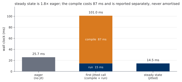
The recorded run: eager \(25.7\) ms, first jitted call \(101.0\) ms of which about \(87\) ms is compilation, steady state \(14.5\) ms.

Any claim in this course about the speed of a JAX function reports compile time separately from steady-state time, and never amortises the compile into the speedup.

The rule exists because the alternative is easy and wrong in both directions. Time the first call and jit looks four times slower than eager. Time only the steady state and quote it as the speedup, and you have hidden a fixed cost that a short-running script never earns back.

Both numbers together say something a single number cannot: on this workload jit is \(1.8\) times faster per call and costs \(87\) ms up front, so it pays for itself after about eight calls and is a loss below that.

Two more honesties, since this is the block about them.

A factor of \(1.8\) is a modest speedup, and it is the real one. This workload is a chain of matrix multiplications, and a matrix multiplication is already a call into a tuned kernel with little for a compiler to improve. XLA earns its large factors by fusing many small operations, and there are few small operations here. Reporting \(1.8\) where you hoped for \(20\) is the entire point of measuring.

Wall-clock time does not reproduce, and the notes will not pretend it does. Every other number on this page comes back identical on a re-run. These three do not: they move by several milliseconds between runs on an unloaded machine, and they will be different on yours. What reproduces is the shape — compilation dominates the first call, steady state beats eager, break-even is on the order of ten calls. The script reports the median of many calls for that reason, and the recorded run is in u0l5_solvers.json. Quote a timing with the machine it was measured on, or do not quote it.

F · Freeze, packet, and PS0

The freeze

common/odesolve.py and jax-primer.ipynb are frozen at the end of this session, and tagged u0l5-freeze. U3.L1 imports odeint under the contract of Section 2, so a change to that signature after today is a breaking change and needs a dated note.

The packet

The self-study packet that PESC students receive at enrollment is assembled from what this unit produced:

• the ode-solver-notes of U0.T5, which were written standalone-first for this purpose;
• jax-primer.ipynb and lab-u0l5.ipynb, with their solutions;
• a pointer list into UP.A for the probability that the joint sessions assume;
• a README with a suggested pacing of three evenings.

The packet exists because of a rule from the top of the course: no joint session may require having attended U0. The packet and UP.A are the sanctioned onboarding surface, and everything else has to stand without them.

PS0

PS0 is assigned now, and it is a synthesis rather than a new topic. Every piece of it is something you built.

Train your VAE (vae-mnist-scratch, U0.L3) using your U-Net (unet-skeleton, U0.L4) as the encoder, with the hygiene-stack (U0.L2), and evaluate it with your eval-harness (U0.L4): FID at the course-standard sample count, plus sample panels.

Graded on correctness and reproducibility, not on sample quality.

The grading rule is the guardrail, and it is meant literally. A run that is reproducible and produces mediocre samples scores above a run that produces beautiful samples and cannot be repeated. “Reproducible” here has an operational definition, and it is the one the hygiene stack already enforces: the config, the seed, the commit hash with its dirty flag, and the MLflow run. If those four are present and the run comes back, the requirement is met.

There is also a compute ceiling, stated on the assignment. Nothing in PS0 needs more than a single consumer GPU for a small number of epochs, and a submission that needed more than that has misread the exercise.

The bootcamp, closed

Five weeks, and every session produced something that a later session imports.

Table 3: The toolbox, photographed before the road trip.

Artifact	Built in	Consumed by
training-loop-template	U0.L1	every lab, through the hygiene stack
hygiene-stack	U0.L2	every lab; PS0 by name
elbo-derivation	U0.T3	U3.T2, U5.T1
vae-mnist-scratch	U0.L3	U0.L4, PS0
time-conditioning-patterns	U0.T4	U0.L4, the U3 labs, U5.T1
fid-definition	U0.T4	U0.L4
unet-skeleton	U0.L4	U3.L2, U3.L3, PS0
eval-harness	U0.L4	U1.L2, U3.L2, U3.L3, PS0
ode-solver-notes	U0.T5	U2.L1, U3.L1, the packet
ode-solvers-scratch	U0.L5	U3.L1, the packet
jax-primer	U0.L5	the JAX moments; the packet

None of Table 3 is generative modelling. All of it is what generative modelling is built out of, and from the next unit onward the course stops building tools and starts using them.

The next live session is UP.T1, where the course proves the one result it uses three times: conditional expectation as an \(L^2\) projection — the projection Lemma. Everything after it leans on that page.

References

Kidger, Patrick. 2022. “On Neural Differential Equations.” PhD thesis, University of Oxford. https://arxiv.org/abs/2202.02435.