U0.L5 — Solvers by Hand and a JAX Crash Course

Flow-Based Generative Models · UFRJ · 2026.2

01The tour

Two builds, and who imports them

Artifact	Who imports it
common/odesolve.py	U3.L1 — ODE sampling
jax-primer.ipynb	the JAX moments of U1.L1, U2.L1, U3.L1

Both also ship in the PESC self-study packet.

The first samples of this course’s first Flow Matching model will be drawn by the file you write in the next 25 minutes.

Two minutes, and the frame has to land: today’s output is not a result, it is infrastructure — the same framing as U0.L4. Say the U3.L1 line slowly. It is true and it is the whole motivation for taking the solver seriously.

You are writing onboarding material

Some readers of your notebook will be PESC students who were not in this room, with no lecturer to ask.

So: full prose between cells, a self-check after every TODO, and the solutions ship with the packet.

Write for colleagues you have not met.

The dual-use rule made motivating rather than bureaucratic. This is also straightforwardly good practice — the reader who is not here includes you, in six months.

Why JAX at all

1. grad / vmap / jit make several course constructions clearer than the PyTorch version
2. diffrax is the strongest ODE library in the ecosystem
3. Reading JAX is now a research-literacy requirement

PyTorch stays primary. JAX moments are mirrors, never the only path.

Say the argument out loud so the choice is legible. Point 1’s concrete case is per-sample Jacobians for the coupling-layer log-dets in U1.L1 — they arrive in block D as a TODO.

02The solver module

The contract — frozen today

odeint(f, x0, t0, t1, method="rk4",
       n_steps=None, rtol=None, atol=None,
       return_traj=False)
    -> x1          # Tensor carrying .nfe
    -> (ts, xs)    # if return_traj=True

1. f(t, x) — time first
2. x0 is (B, d) — batched by construction
3. every call reports its NFE

Read the three laws off the slide, do not elaborate yet. The next three slides are the elaborations, one law each.

Law 1 — time first, because they said so

torchdiffeq and diffrax both take f(t, y).

The two orderings are equally arbitrary in isolation. Agreeing with the ecosystem is not.

A right-hand side you write today is one the professional libraries accept unchanged — which makes U2.L1 a change of library, not a rewrite.

Recorded in U0.T5 as the binding convention. Worth one sentence on why conventions that are arbitrary are still worth obeying exactly.

Law 2 — the batch is not an afterthought

A generative model is sampled in batches, so the solver takes batches.

Notice what this does not require:

• the step loop is an ordinary Python loop over steps
• the batch dimension is carried by the tensor ops
• there is no vmap in this file, and none is needed

Plant this deliberately. Block D is about the case where you DO need vmap, and the contrast is what makes that case land. A batched loop is not a vmap use.

Law 3 — NFE is a first-class output

NFE is this course’s cost currency.

• U2 watches it grow during training, and it hurts
• U3 is largely about making it small

A solver that hides its NFE cannot be compared with another solver — and a comparison you cannot make is a comparison you will not make.

This is the law people leave out, so it gets the argument. The mechanism is on the next slide.

The cost travels with the answer

class SolverOutput(torch.Tensor):
    nfe: int
    method: str
    accepted: int | None   # adaptive only
    rejected: int | None   # adaptive only

It is a Tensor — prints, indexes, broadcasts like one.

A warning in a docstring does not survive contact with a results table.

Callback to U0.L4, where FIDValue refused a comparison across protocols. Same reasoning: make the metadata travel with the number. Honest caveat to say out loud: the attributes do not survive arithmetic — (x1 - x0).nfe raises.

Four TODOs, three of them transcription

TODO	Method	NFE / step
1	Euler	1
2	Heun	2
3	RK4 (transcribe the tableau)	4
4	Adaptive Heun(2)/Euler(1)	2 / attempt

A tableau is the table of coefficients defining a Runge–Kutta method. We are consumers of tableaux, not designers.

TODOs 1–3 are mechanical on purpose — U0.T5 derived them, and re-deriving them here spends the only 90 minutes in which the code gets written.

Say “on purpose” clearly, or the scaffolding reads as condescension. The interesting part of RK4 is its slope, and that is block C.

TODO 4 — two orders from two evaluations

\(k_1\) alone is the Euler step:

\[ \hat{x}_{n+1} = x_n + h k_1 \qquad x_{n+1} = x_n + \tfrac{h}{2}(k_1 + k_2) \]

Their difference estimates the local error; the step is judged against \(\mathrm{sc}_i = \texttt{atol} + \texttt{rtol}\cdot\max(|x_{n,i}|,|x_{n+1,i}|)\).

Two things that are easy to get wrong, both checked: propagate the higher-order value, and update \(h\) after a rejection too.

The second one is the classic infinite loop: a rejected step that retries at the same size rejects again forever. The controller’s rule is unconditional.

Checkpoint — your own spiral

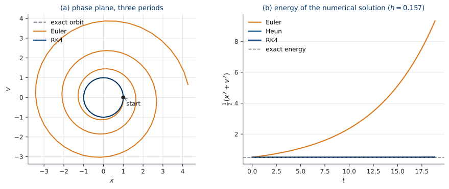
The U0.T5 icon, now self-made. \(h = 2\pi/40\).

The assert is not on the picture: Euler’s energy grows by exactly \(1 + h^2\) per step, and the notebook checks that ratio.

A plausible spiral with the wrong growth factor is a bug the eye does not catch. This is the reason every checkpoint in this notebook asserts a number rather than showing a plot.

The scope is deliberate

This module integrates forward. No adjoint, no differentiation through the solve.

Sampling is inference: no gradient is needed to draw a sample.

Nothing blocks autograd — and what it would cost you in memory is precisely the problem U2.T1 exists to solve.

One sentence and move on. Do not open the adjoint here; it is U2.T1’s whole session. If someone pushes: “U2.T1”.

03The convergence study

Collecting a prediction from U0.T5

Exercise 2 asked you to predict the three slopes before making the plot. The answer was 1, 2, 4.

Now you make the plot with your own solvers.

Measuring the order is how you find a bug in a Runge–Kutta method. A tableau typo usually leaves a method that still converges — at the wrong rate.

Collect the payoff explicitly; they did the work last session. A hand-written RK4 scoring slope 3 has a typo, and nothing else finds it.

The same cost, spent three ways

Method	Steps at NFE \(=4000\)	Error at \(t=2\pi\)
Euler	4000	\(4.9 \times 10^{-3}\)
Heun	2000	\(1.0 \times 10^{-5}\)
RK4	1000	\(8.2 \times 10^{-11}\)

Almost eight orders of magnitude — a factor of \(6\times10^{7}\) — and nobody spent more than anybody else.

Measured with their own module. Then put the question to the room: at an error budget of 1e-4, which row do you pick? That is the decision the NFE table exists to make possible.

The caveat that matters later

The table on the previous slide assumes you want high accuracy.

At a loose tolerance the three methods sit much closer together. At one or two evaluations total, a high-order method has no advantage at all — it has not taken enough steps for its order to express itself.

Sampling a generative model at 4 NFE lives in exactly that regime.

This is why the few-step sampling literature is not simply “use RK4”. Plant it; U3.T4 collects it.

Sweeping the tolerance

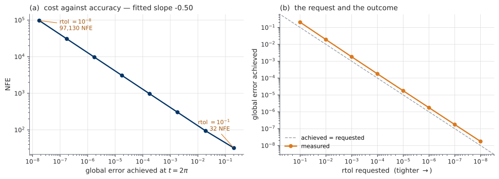
rtol from \(10^{-1}\) to \(10^{-8}\). (a) NFE against error achieved, fitted slope \(-0.50\). (b) The outcome against the request, with the diagonal.

Three readings, next three slides, one each. Do not rush this figure — it is the block’s deliverable and they made it themselves.

Reading 1 — the request is honoured, here

Panel (b) is a straight line parallel to the diagonal.

Nothing guarantees that. The controller bounds a local error estimate; panel (b) plots the global error at the end.

“I set rtol to \(10^{-6}\)” is a statement about what you asked for, never about what you got.

On this problem local and global error are proportional — the good case. On a badly conditioned problem they are not. This distinction is worth 60 seconds.

Reading 2 — the slope is the order

Fitted slope \(-0.50\); an order-2 method predicts \(-1/2\).

Halving the error costs \(\sqrt{2}\) times the work here. With a fifth-order method it would cost \(2^{1/5}\).

Block E measures exactly that difference.

Shrink h by 10^(1/2) to cut local error by 10; NFE goes as 1/h. Forward-point to the diffrax comparison so it does not arrive as a surprise.

Reading 3 — rejections are rare, and should be

Across all eight runs: \(0, 0, 1, 1, 2, 3, 3, 4\) rejected steps — out of up to 48 561 accepted.

The safety factor \(0.9\) is what buys that.

A rejected step costs its evaluations and makes no progress. A controller that rejects constantly is misconfigured.

Rejection is not failure — it is the controller working. But rarely.

The two failure smells, on their own plot

Left end: 32 evaluations, error \(0.2\) on an orbit of radius \(1\). Fast, smooth, plausible, wrong. Nothing complained.

Right end: 97 130 evaluations, error \(1.8\times10^{-8}\), cost \(\times 3035\). You notice immediately; it costs only time.

The test for “too loose”: halve both tolerances and re-run. If the answer moves by more than you can accept, the original was not converged. Say that the dangerous failure is the silent one — this recurs for the rest of the course.

04JAX in five moves

One sentence, then five elaborations

JAX is NumPy, plus function transformations, plus explicit randomness.

Scope, declared. Five moves and stop. No flax, no optax beyond a mention. No sharding, no TPU.

The primer optimizes for reading research JAX and mirroring this course. Not for writing production JAX.

Declaring scope protects the 28 minutes. If someone asks about flax: “U3.L1’s JAX moment, one cell”.

Move 1 — pure functions and jnp

y = x.at[i].set(v)   # new array; x unchanged

You give up in-place mutation. What you buy is that the function can be transformed — differentiated, vectorized, compiled, or all three.

A transformation must know that calling your function twice with the same arguments does the same thing twice.

Purity is the price of transformability.

One honest paragraph, as the plan says. Do not apologise for the price and do not oversell the purchase — the next four slides are the purchase.

Move 2 — grad returns a function

def loss(theta, x):
    return jnp.sum((theta * x - 1.0) ** 2)

dloss = jax.grad(loss)      # same signature
g = dloss(theta, x)         # same pytree as theta

No tape. No .backward(). No .grad attribute on anything.

value_and_grad gives both outputs for the price of one — mention it, they will want it in every training loop they write.

The ritual, third appearance

\[ \frac{\partial f}{\partial \theta_i} \;\approx\; \frac{f(\theta + \varepsilon e_i) - f(\theta - \varepsilon e_i)}{2\varepsilon} \]

U0.L1 introduced it. U0.L2 repeated it. By now it should be a reflex.

Three lines, one second, and it is the only thing that distinguishes a gradient from a plausible array of numbers.

Third appearance is the point of the slide. Say it as a habit being installed, not as a new technique.

Move 3 — vmap, and why it exists

per_sample = jax.vmap(
    jax.grad(loss_one), in_axes=(None, 0, 0)
)(params, xs, ys)

loss_one is the loss of one sample — no batch dimension anywhere in its body.

in_axes=(None, 0, 0): parameters shared, inputs and targets mapped.

This TODO was chosen because per-sample gradients are genuinely awkward in eager PyTorch, and the awkwardness is why people never look at them. The next slide is what looking at them shows.

What per-sample gradients look like

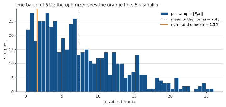
Dotted: mean of the norms, \(7.48\). Solid: norm of the mean, \(1.56\).

The gap is cancellation, and it is what averaging a batch is. But the number the optimizer sees is not a typical sample’s number.

Spread runs from 0.003 to 26.0 — a factor of nearly 10^4, invisible from the batch gradient alone. Then say the check: vmap(grad) against a Python loop over grad deviates by exactly zero. vmap is not an approximation of the loop.

Where this returns

U1.L1 computes a coupling layer’s Jacobian log-determinant, per sample, with jax.jacfwd.

Same composition, different inner transformation.

This TODO is its warm-up.

Forward pointer only. Do not open coupling layers — that is U1’s session.

Move 4 — jit, in three sentences

1. JAX runs your Python once, with placeholders, and records the operations. The recording is compiled.
2. The recording is cached per shape and dtype — a new shape re-traces.
3. Python control flow branching on a value cannot be recorded.

Eager is the other mode: each operation runs as the interpreter reaches it. That is the baseline block E times against.

Three sentences is the whole tracing model they need today. Do not go further into jaxpr — it is not needed to read research code.

The trap, planted rather than described

@jax.jit
def f(x):
    if x > 0:        # TracerBoolConversionError
        return x
    return -x

Run the cell. Read the error. Then fix it with jnp.where.

An error message you have met once is a different thing from an error message you have read about.

Give them 90 seconds to actually hit it. This is the first error every newcomer to JAX meets, and meeting it here is cheaper than meeting it in U3.L1.

Move 5 — pytrees and explicit keys

key = jax.random.key(0)
key, sub = jax.random.split(key)   # never reuse
x = jax.random.normal(sub, (batch, d))

No global seed. No hidden state. Same key, same value, always.

A pytree is any nest of containers with arrays at the leaves; params are a dict of dicts. grad of a loss over that dict returns a dict of the same shape, and tree_map applies an update across the whole nest.

Randomness as an argument

U0.L2 made reproducibility a discipline: seed three generators, record the seed, remember not to disturb the stream.

Here it is not a discipline. A key you forgot to split is a bug you can see in the code, and a function’s randomness is visible in its signature.

JAX makes the seeding discipline structural.

This is the slide that ties the primer back to the course’s own obsession. Randomness is an argument; reproducibility is the default.

05The same ODE in diffrax

The adapter is two lines

def harmonic_jax(t, y, args):
    return jnp.array([y[1], -y[0]])

sol = diffrax.diffeqsolve(
    diffrax.ODETerm(harmonic_jax),
    diffrax.Tsit5(), t0=0.0, t1=T, dt0=0.01,
    y0=y0,
    stepsize_controller=diffrax.PIDController(
        rtol=1e-6, atol=1e-8),
)

Every argument is one you now understand (Kidger 2022).

Tsit5 = order-5 tableau with an embedded order-4 estimate — TODO 4 with better coefficients and more stages. PIDController = their controller with a more careful smoothing law. dt0 is the first step, which the controller overrides.

The cross-check

Two independent solvers, one problem. If they disagree, one of them is wrong.

diffrax Tsit5 at rtol \(=10^{-12}\), against your RK4 at 4000 fixed steps:

\[ \bigl\| x^{\text{diffrax}}_1 - x^{\text{yours}}_1 \bigr\| \;=\; 4.1 \times 10^{-13} \]

Your solver is correct. Now the rest of the news.

Let “your solver is correct” land before turning the page. The next slide is the humility, and it works only if the correctness landed first.

A factor of 270

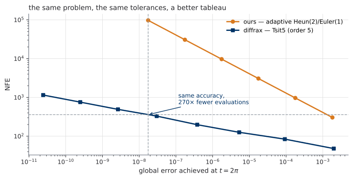
The adaptive Heun of block B against diffrax’s Tsit5, same problem, same tolerances. At error \(1.8\times10^{-8}\): 97 130 evaluations against about 360.

The lines are diverging — an order-5 cost curve is flatter than an order-2 one.

Read it twice. First reading: humility. Their solver is correct and 270x more expensive than a specialist’s. Second reading: continuity — U2.L1 uses diffrax and torchdiffeq as the professional mirrors and re-explains none of it.

Writing it was still necessary

You now know what Tsit5, rtol and PIDController mean — and you know it because you built the smaller version of each.

The from-scratch pass is how you learn the object. It is not how you integrate an equation you care about.

This is the course’s standing position on from-scratch implementation, stated where the evidence for it is on the previous slide. It recurs in U1, U2 and U3.

Honest timing

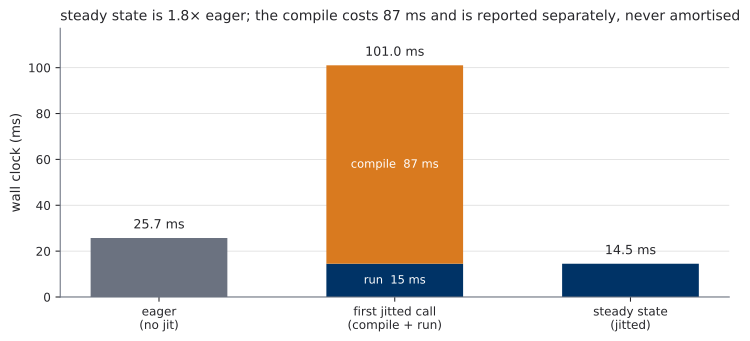
CPU, JAX 0.10.2 — one machine, one run.

Report compile time separately from steady-state time. Never amortise the compile into the speedup.

Recorded run: eager 25.7 ms, first call 101.0 ms of which ~87 ms compiles, steady 14.5 ms. The rule is a course standard from here on, and U2.L1’s plan already assumes it.

Both numbers, or neither

Time the first call, and jit looks four times slower.

Time only the steady state, and you have hidden a fixed cost a short script never earns back.

Together: \(1.8\times\) faster per call, \(87\) ms up front — break-even after about eight calls, a loss below that.

Neither number alone is a lie exactly; each alone is unusable. That is the argument for the rule.

Two more honesties

\(1.8\times\) is modest, and it is the real number. This workload is matrix multiplications — already tuned kernels, little for a compiler to fuse. XLA earns its large factors on many small operations.

Wall clock does not reproduce. Every other number today comes back identical. These three move by milliseconds between runs, and will differ on your machine.

Reporting 1.8 where you hoped for 20 is the entire point of measuring. What reproduces is the shape: compile dominates the first call, steady beats eager, break-even is around ten calls. Quote a timing with its machine or not at all.

06Freeze, packet, PS0

Frozen and tagged

common/odesolve.py and jax-primer.ipynb, tagged u0l5-freeze.

U3.L1 imports odeint under today’s contract. A change to that signature after today is a breaking change.

Same discipline as U0.L4’s two freezes. Say the tag out loud so it exists in their notes.

The packet

• ode-solver-notes (U0.T5 — written standalone-first for this)
• jax-primer.ipynb + lab-u0l5.ipynb, with solutions
• a pointer list into UP.A for the probability assumed
• a README with a three-evening pacing

It exists because of a rule from the top of the course: no joint session may require having attended U0.

The packet and UP.A are the sanctioned onboarding surface. Everything else has to stand without them — that is the PESC parity protocol.

PS0 — assigned now

Your VAE (U0.L3) with your U-Net (U0.L4) as encoder, trained with the hygiene stack (U0.L2), evaluated with your harness (U0.L4): FID at the course-standard \(n\), plus panels.

Graded on correctness and reproducibility, not on sample quality.

Every piece of PS0 is something they already built. It is a synthesis, not a new topic. Say the grading rule twice.

The guardrails, literally

A run that is reproducible and mediocre scores above a run that is beautiful and cannot be repeated.

“Reproducible” is operational — the hygiene stack already enforces it:

config · seed · commit hash + dirty flag · the MLflow run

Compute ceiling: a single consumer GPU, a small number of epochs. More than that has misread the exercise.

The ceiling exists so nobody buys cloud credits for a bootcamp assignment. If someone’s plan needs more, their plan is wrong, not their hardware.

Five weeks, eleven artifacts

Artifact	Built	Consumed by
training-loop-template	L1	every lab
hygiene-stack	L2	every lab; PS0
elbo-derivation	T3	U3.T2, U5.T1
vae-mnist-scratch	L3	L4, PS0
time-conditioning-patterns	T4	L4, U3 labs, U5.T1
fid-definition	T4	L4
unet-skeleton	L4	U3.L2, U3.L3, PS0
eval-harness	L4	U1.L2, U3.L2/L3, PS0
ode-solver-notes	T5	U2.L1, U3.L1, packet
ode-solvers-scratch	L5	U3.L1, packet
jax-primer	L5	JAX moments, packet

The toolbox photographed before the road trip. None of it is generative modelling; all of it is what generative modelling is built out of.

From here, the course uses its tools

The next live session is UP.T1, where the course proves the one result it uses three times:

conditional expectation as an \(L^2\) projection — the projection Lemma.

Everything after it leans on that page.

Rest during the async window. The PESC students are just arriving.

Close warmly and close the unit. Point at the packet one last time: it is their best review document too, because it was written for someone with no lecturer.

References

Kidger, Patrick. 2022. “On Neural Differential Equations.” PhD thesis, University of Oxford. https://arxiv.org/abs/2202.02435.