U0.T2 — Making Training Work
Session U0.T2 · date: see calendar-map
These notes install the practical stack the whole course trains with: the optimizer telescoping SGD → momentum → Adam → AdamW, the warmup + cosine learning-rate schedule, initialization by variance propagation, the right normalization for generative models, residual connections, and the CNN’s inductive bias. The session’s deliverable is the recipe card at the end (Section 7), the artifact optimizer-schedule-defaults. From U0.L2 onward, “train with the U0.T2 defaults” refers to that box, and every later lab (flows, CFM, DDPM-as-a-special-case) cites it instead of re-deciding.
One framing rule governs the whole session: every topic here is justified by its reappearance later in the course, and we say so explicitly each time. Standing references for the unit: (Bishop and Bishop 2024; Murphy 2023).
The hook: same code, three seeds
U0.L1 ended with an unmarked homework-lite: re-run the two-moons training with three seeds and eyeball the variance. Here is that experiment, run properly:
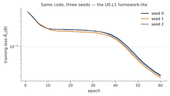
On this toy problem the variance is only annoying. In a badly configured run (wrong learning rate, bad init, wrong normalization) the same variance decides whether training converges at all. The question of the day: which training settings make training reliably work, and what are our defaults? The answer, literally, is Section 7.
Optimizers: the telescoping SGD → momentum → Adam → AdamW
SGD and the minibatch gradient
Full-batch gradient descent on the empirical risk \(\widehat{R}_n(\theta)\) (U0.T1) costs a full pass over the dataset per parameter update. Stochastic gradient descent replaces the full gradient by a minibatch estimate. One piece of notation first, because it carries the whole course’s loss functions: the empirical measure.
For a minibatch \(B \subset \{1, \dots, n\}\), the empirical measure of the minibatch is the discrete probability distribution \[ \widehat{q}_B \;=\; \frac{1}{|B|} \sum_{i \in B} \delta_{(x_i,\, y_i)}, \] which puts mass \(1/|B|\) on each sampled pair \((x_i, y_i)\) (here \(\delta_z\) is the point mass at \(z\)). Sampling from \(\widehat{q}_B\) means picking one of the batch’s pairs uniformly, and an expectation under \(\widehat{q}_B\) is nothing more than the average over the batch. The minibatch loss and SGD update are \[ \begin{aligned} \mathcal{L}_B(\theta) &\;=\; \mathbb{E}_{(x,y)\sim \widehat{q}_B}\big[\ell\big(f_\theta(x),\, y\big)\big] \;=\; \frac{1}{|B|} \sum_{i \in B} \ell\big(f_\theta(x_i),\, y_i\big), \\[4pt] \theta_{k+1} &\;=\; \theta_k - \eta_k\, g_k, \qquad g_k = \nabla_\theta\, \mathcal{L}_{B_k}(\theta_k), \end{aligned} \] with \(\eta_k > 0\) the step size (learning rate) at step \(k\).
The same construction with all \(n\) samples gives \(\widehat{q}_n\), the empirical measure of the full dataset, and U0.T1’s empirical risk is exactly \(\widehat{R}_n(\theta) = \mathbb{E}_{(x,y)\sim \widehat{q}_n}[\ell(f_\theta(x), y)]\). The notation buys us one uniform language: every loss in this course, from today’s classifier to the final flow-matching objective, is an expectation with its sampling distribution written under the \(\mathbb{E}\).
Two facts carry the section. First, unbiasedness: with \(B\) sampled uniformly, \(\mathbb{E}_B[g] = \nabla_\theta \widehat{R}_n(\theta)\), so the noisy gradient points the right way on average. Second, the noise scale. Across random draws of the minibatch, \(g\) scatters around its mean, and the covariance matrix \(\operatorname{Cov}_B[g]\) quantifies that scatter, exactly as a variance quantifies the scatter of a scalar estimator. Since \(g\) is an average of \(|B|\) independent per-sample gradients, its covariance is the single-sample covariance divided by \(|B|\): \[ \operatorname{Cov}_B[g] \;\approx\; \frac{1}{|B|}\, \Sigma(\theta), \qquad \Sigma(\theta) = \operatorname{Cov}_{(x,y)\sim \widehat{q}_n}\!\big[\nabla_\theta\, \ell\big(f_\theta(x),\, y\big)\big], \] where \(\Sigma(\theta)\) is the covariance of one sample’s gradient around the full-data gradient. (The \(\approx\) hides the finite-population correction from sampling without replacement; it is negligible for \(|B| \ll n\).) Typical fluctuations therefore shrink like \(1/\sqrt{|B|}\). Small batches are cheap and noisy (with some empirically documented regularizing jitter); large batches are clean and hardware-efficient but do not buy proportionally fewer steps. The noise never vanishes; it is why the loss curves in the hook figure wiggle. Our practical stance, encoded in the recipe card: batch size is chosen by memory and always reported.
Note the notation discipline, which extends U0.T1’s rule to optimizer pseudocode: even the minibatch loss carries its sampling subscript. There are no unsubscripted expectations in this course, optimizers included.
The enemy is ill-conditioning
The picture that motivates everything after plain SGD:
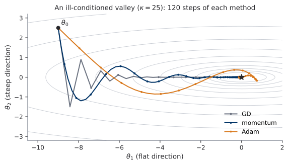
A loss surface whose curvature differs wildly across directions is ill-conditioned; for deep networks the effective condition number is astronomically worse than this toy’s \(\kappa = 25\), and the directions are not axis-aligned. Plain GD’s single global step size must be safe in the steepest direction, hence wasteful in all the flat ones.
Momentum: an exponential moving average of gradients
\[ m_k \;=\; \beta\, m_{k-1} + (1-\beta)\, g_k, \qquad \theta_{k+1} \;=\; \theta_k - \eta\, m_k, \qquad \beta \approx 0.9. \]
The recursion makes \(m_k\) an exponential moving average (EMA) of past gradients: components that oscillate step-to-step (across the valley) cancel in the average; components that persist (along the valley floor) accumulate. That is the heavy-ball intuition: a ball with inertia does not reverse direction on every bump. Two bookkeeping remarks. PyTorch’s SGD(momentum=0.9) implements the un-normalized recursion \(m_k = \beta m_{k-1} + g_k\), which traces the same trajectory family with a rescaled learning rate. And Nesterov momentum (gradient evaluated at a look-ahead point) is named here so you recognize the checkbox, and not derived.
Adam: two EMAs and a per-coordinate step size
Adam maintains EMAs of both the gradient and its elementwise square: \[ \begin{aligned} m_k &= \beta_1\, m_{k-1} + (1-\beta_1)\, g_k &&\text{(first moment: direction)}\\ v_k &= \beta_2\, v_{k-1} + (1-\beta_2)\, g_k^{\,2} &&\text{(second moment: scale, per coordinate)}\\ \widehat{m}_k &= \frac{m_k}{1-\beta_1^{\,k}}, \qquad \widehat{v}_k = \frac{v_k}{1-\beta_2^{\,k}} &&\text{(bias correction)}\\ \theta_{k+1} &= \theta_k - \eta_k\, \frac{\widehat{m}_k}{\sqrt{\widehat{v}_k} + \varepsilon} &&(\beta_1 = 0.9,\; \beta_2 = 0.999,\; \varepsilon = 10^{-8}). \end{aligned} \] The step \(\eta_k / (\sqrt{\widehat{v}_k} + \varepsilon)\) is per coordinate: parameters with historically large gradients take small steps and vice versa. This addresses exactly the two diseases above: ill-conditioning (each direction gets its own effective step size), and gradient scale disparity across layers and parameter types (embeddings vs. biases vs. conv kernels), which no single global \(\eta\) can serve.
The race is worth watching once: GD’s step-by-step alternation in the steep coordinate, momentum’s average visibly rotating toward the valley axis, and Adam’s two per-coordinate step-size bars diverging (flat coordinate long, steep coordinate short) while its iterate moves at a uniform rate in both directions. The dynamics are numerically identical to the static figure above:
The bias-correction factors were the session’s live derivation, reproduced in full:
The EMAs start at \(m_0 = 0\), so early estimates are biased toward zero. Unrolling the recursion, \[ m_k \;=\; (1-\beta)\sum_{i=1}^{k} \beta^{\,k-i}\, g_i . \] If the gradient distribution is approximately stationary over the averaging window, \(\mathbb{E}_B[g_i] \approx g\) for all \(i \le k\), then by linearity and the geometric sum, \[ \mathbb{E}_B[m_k] \;\approx\; g\,(1-\beta)\sum_{i=1}^{k} \beta^{\,k-i} \;=\; g\,(1-\beta)\,\frac{1-\beta^{\,k}}{1-\beta} \;=\; g\,\big(1-\beta^{\,k}\big). \] Hence \(\widehat{m}_k = m_k / (1-\beta^{\,k})\) satisfies \(\mathbb{E}_B[\widehat{m}_k] \approx g\): the startup bias is removed, and since \(\beta^{\,k} \to 0\) the correction retires as training proceeds. The same computation with \(\beta_2\) and \(g_i^{\,2}\) gives the second-moment factor. \(\square\)
Note for Section 3: the derivation assumed the estimates are meaningful once corrected. But at step 10, \(\widehat{v}_k\) is an average of ten squared gradients drawn at a rapidly moving \(\theta\). Bias correction fixes the systematic error, not the statistical one. That residual unreliability is what warmup exists to survive.
AdamW: decoupled weight decay
First, the vocabulary. L2 regularization (also ridge or Tikhonov regularization) adds the penalty \(\frac{\lambda}{2}\lVert\theta\rVert_2^2\) to the loss; since \(\nabla_\theta \frac{\lambda}{2}\lVert\theta\rVert_2^2 = \lambda\theta\), its effect on plain gradient descent is to shrink every weight by \(\eta\lambda\theta\) per step, which is why the same operation is also called weight decay. In classical SGD the two descriptions (penalty in the loss, shrinkage in the update) are the same thing.
Under adaptive steps they diverge. If \(\lambda\theta_k\) is added to the gradient, it enters both EMAs and is divided by \(\sqrt{\widehat{v}_k}\) like everything else: coordinates with large historical gradients are barely regularized, and the effective decay strength becomes an accident of gradient history. AdamW decouples the decay from the adaptive machinery: \[ \theta_{k+1} \;=\; \theta_k - \eta_k \left( \frac{\widehat{m}_k}{\sqrt{\widehat{v}_k} + \varepsilon} \;+\; \lambda\, \theta_k \right), \] so every coordinate decays at the same rate \(\eta_k \lambda\), as the regularizer intended. Standard practice, adopted in the recipe card: normalization parameters (\(\gamma, \beta\) below) and embeddings are excluded from weight decay, because shrinking a scale parameter toward zero is not regularization, it is sabotage.
The course optimizer is AdamW. Every training run from U0.L2 through U3 uses it with the recipe-card defaults; deviations must be justified in writing.
One honest paragraph to set expectations. On vision classification benchmarks, carefully tuned SGD + momentum often generalizes slightly better than Adam-family optimizers; that literature is real and worth knowing. Nobody trains modern large generative models that way: time-conditioned objectives, where a single batch of a later loss \(\mathbb{E}_{t,\, x_1\sim q,\, x\sim p_t(\cdot\mid x_1)}\!\left[\cdots\right]\) mixes time steps with wildly different gradient scales, are exactly the regime where per-coordinate adaptivity earns its keep. Our default is chosen for the models we build, not as a universal claim.
Why this matters later. Every flow / CFM / DDPM lab in this course (U1.L1 through U3.L3) trains with AdamW under the recipe-card defaults, and PS0 requires them by name.
Schedules: warmup + cosine
The learning rate is not one number; it is a schedule \(\eta_k\), indexed by the training step. Terminology, fixed once for the whole course: a step (the \(k\) above) is one optimizer update on one minibatch; an epoch is a full pass over the dataset, roughly \(n/|B|\) steps. They are not interchangeable, and every schedule in this course is defined per step, because that is what the optimizer state (\(m_k\), \(v_k\), and the estimates’ reliability) actually evolves in. The course default schedule has two phases, both justified above.
Warmup. Adam’s update divides by \(\sqrt{\widehat{v}_k}\), and for small \(k\) the second-moment estimate is built from a handful of squared gradients evaluated at a rapidly moving, randomly initialized \(\theta\): bias-corrected, but statistically garbage. Dividing by the square root of garbage makes some coordinates take enormous steps precisely when the network is least able to absorb them; the classic symptom is a loss spike or NaN within the first few hundred steps. The fix is operational, not aesthetic: ramp \(\eta_k\) linearly from \(\approx 0\) while the moment estimates fill up. Practical sizing: warmup over roughly 1–5% of total training steps.
Cosine decay. After warmup, decay the learning rate smoothly to approximately zero following a half-cosine. Three virtues: it is smooth (no step-function shocks to the moment estimates), it has essentially one parameter (the total step count), and it spends the end of training at a tiny learning rate, polishing rather than wandering. Combined: \[ \eta_k \;=\; \begin{cases} \eta_{\max}\, \dfrac{k}{K_w}, & k \le K_w \quad \text{(linear warmup)},\\[2ex] \dfrac{\eta_{\max}}{2} \left(1 + \cos\!\left(\pi\, \dfrac{k - K_w}{K - K_w}\right)\right), & K_w < k \le K \quad \text{(cosine decay)}, \end{cases} \] with \(K\) the total number of steps and \(K_w\) the warmup horizon (both counted in steps, not epochs).
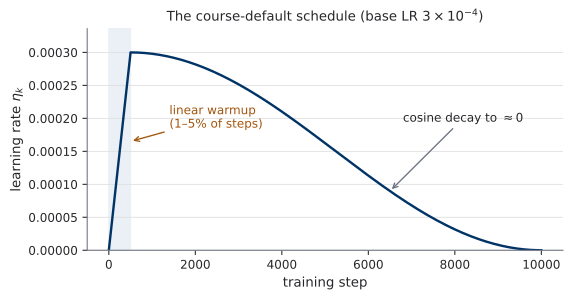
Linear warmup over 1–5% of total steps, then cosine decay to \(\approx 0\). Later labs assume this silently; anything else must be justified in writing.
Why this matters later. Time-conditioned generative models are noisy-gradient regimes: the loss samples \(t\) afresh each batch, so gradient scale and direction fluctuate more than in supervised training. Warmup + cosine is the schedule the U3 labs assume without comment.
Initialization
The failure mode
Depth multiplies scales. If each layer multiplies the typical activation magnitude by a factor \(c \neq 1\), then depth \(L\) produces \(c^L\): geometric growth or geometric death, in the forward pass and, by the chain rule through the same weight matrices, in the backward pass too. The empirical picture:
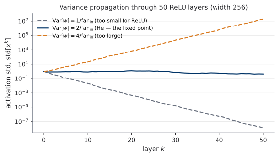
At depth 50, the wrong constant costs a factor of \(10^{7}\). No learning rate rescues a network whose signals have died or exploded before the first gradient step.
Variance propagation, derived
The session’s second live derivation: light, and boxed because U0.L2’s debugging exercise leans on it.
Let \(y = W x\) with \(W \in \mathbb{R}^{m \times d}\), entries i.i.d. with \(\mathbb{E}[w_{ij}] = 0\) and \(\operatorname{Var}[w_{ij}] = \sigma_w^2\), independent of \(x\), whose coordinates are i.i.d. with mean \(0\) and variance \(\operatorname{Var}[x]\). Then for each output coordinate, \[ \operatorname{Var}[y_i] \;=\; \operatorname{Var}\!\Big[\sum_{j=1}^{d} w_{ij}\, x_j\Big] \;=\; \sum_{j=1}^{d} \operatorname{Var}[w_{ij}\, x_j] \;=\; d\, \sigma_w^2 \operatorname{Var}[x], \] using independence and \(\mathbb{E}[w_{ij}] = 0\). A ReLU halves the second moment of a symmetric input, \(\mathbb{E}\big[\operatorname{ReLU}(z)^2\big] = \tfrac{1}{2}\, \mathbb{E}[z^2]\) (the negative half-line’s mass is zeroed). One linear + ReLU layer therefore maps \[ \operatorname{Var}[x] \;\longmapsto\; \tfrac{1}{2}\, d\, \sigma_w^2\, \operatorname{Var}[x], \] and the activation scale is preserved across depth iff the per-layer factor is 1: \[ \sigma_w^2 \;=\; \frac{2}{\text{fan}_{\text{in}}} \qquad \text{(He initialization, ReLU family)}. \] For tanh/linear layers (no ReLU halving), the analogous condition is \(\sigma_w^2 = 1/\text{fan}_{\text{in}}\); Xavier/Glorot initialization, \(\sigma_w^2 = 2/(\text{fan}_{\text{in}} + \text{fan}_{\text{out}})\), compromises between the forward and backward conditions. Stated without derivation.
Initialization in practice
Three notes that save real debugging time.
- Framework defaults are not what papers assume. PyTorch’s
nn.Lineardefault is not He initialization (it draws from a uniform distribution scaled by \(1/\sqrt{\text{fan}_{\text{in}}}\), a Xavier-flavored choice predating the ReLU analysis). When reproducing a paper, check what the code actually does; when writing course code, set the init explicitly. - Zero-init the last layer whenever “output \(\approx 0\) at start” is sensible: the network then begins as (near) the zero function and training grows it from there, rather than fighting a random function. For the velocity fields \(u_t^\theta\) we train from U3.L1 on, small outputs at init demonstrably calm early training. The same idea returns, dressed up, as adaLN-zero in the DiT preview (U0.T4).
- Residual branches interact with init: zero-initializing the last layer of each residual branch makes the whole block start as the identity, a common and effective recipe (and a hint of why residual networks train so well; see Section 5).
Why this matters later. U0.L2’s sabotaged runs include a bad-init variant: you will be handed loss curves and asked to name the disease from the shapes alone. The figure above (flat vs. dying vs. exploding) is the diagnostic chart.
Normalization and residual connections
What normalization buys, honestly
BatchNorm was introduced (2015) with the story that it fixes internal covariate shift, the drift of layer-input distributions during training. The explanation did not survive later scrutiny; the method did. What normalization demonstrably provides: substantially higher usable learning rates, reduced sensitivity to initialization (the disease of Section 4 treated at run time rather than init time), and an empirically smoother optimization landscape, with the precise mechanism still debated. We treat normalization as engineering with well-documented benefits, not as theory.
The three normalizers
\[
\mu_c = \mathbb{E}_{(x,y)\sim \widehat{q}_B}[x_c],
\qquad
\sigma_c^2 = \operatorname{Var}_{(x,y)\sim \widehat{q}_B}[x_c],
\qquad
\text{BN}(x_c) = \gamma_c\, \frac{x_c - \mu_c}{\sqrt{\sigma_c^2 + \varepsilon}} + \beta_c,
\] with learned scale/shift \(\gamma_c, \beta_c\) and statistics taken over the batch and all spatial positions. Train mode uses the current batch’s statistics (keeping running averages on the side); eval mode uses the running averages, so a single sample can be processed. Two behaviors, one module: model.train() vs. model.eval(); forgetting the switch is a classic silent bug.
BatchNorm’s statistics couple every sample to its batchmates, and this is a genuine liability in three regimes: small batches (noisy statistics: the normalization itself injects noise and the train/eval gap grows), pointwise evaluation (there is no batch; the running averages must faithfully stand in), and, decisive for this course, models conditioned on a per-sample time \(t\). A generative model’s batch mixes samples at \(t \approx 0\) (essentially noise) with samples at \(t \approx 1\) (essentially data); their activation statistics should differ, and batch-normalizing across them couples exactly what the model must keep apart.
LayerNorm and GroupNorm compute the same affine-normalize pattern but take their statistics within a single sample: LayerNorm over all channels (and spatial positions), GroupNorm over contiguous channel groups (typically 32 groups). No batch coupling, no running averages, no train/eval split.
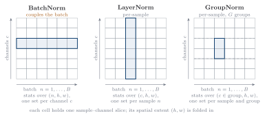
| statistics over | per | train/eval split | in this course | |
|---|---|---|---|---|
| BatchNorm | batch + spatial | channel | yes (running stats) | bootcamp CIFAR-10 classifier only |
| LayerNorm | channels + spatial | sample | no | transformers / DiT (U0.T4, U5) |
| GroupNorm | channel group + spatial | sample, group | no | U-Nets (U0.L4, U3 labs) |
Generative models in this course use GroupNorm (U-Nets) or LayerNorm (transformers). BatchNorm appears in exactly one place: this bootcamp’s CIFAR-10 classifier (U0.L2), where batches are large and evaluation is batched.
Why this matters later. The unet-skeleton you build in U0.L4 is GroupNorm + SiLU throughout; the DiT preview (U0.T4) is LayerNorm + adaLN. Both choices trace back to this section’s knife: per-sample time conditioning is incompatible with batch statistics.
Residual connections
Even with correct init and normalization, plain deep stacks degrade: past a few dozen layers, adding depth hurts training loss, an optimization failure rather than overfitting. The fix is one plus sign: \[ x_{k+1} \;=\; x_k + f_k(x_k). \] The gradient-highway argument is one line: the block’s Jacobian is \[ \frac{\partial x_{k+1}}{\partial x_k} \;=\; I + \frac{\partial f_k}{\partial x_k}, \] and the identity term gives the backward cotangent (U0.T1’s VJP sweep) a direct path through every block. Products of Jacobians along the depth no longer behave like the bare geometric chain of Section 4; the network is free to make each \(f_k\) a small correction rather than a full transformation. Residual connections are what make 50-block U-Nets and 30-block DiTs trainable, and they are in every architecture this course builds from U0.L4 onward.
Keep this innocuous plus sign in mind. In U1.T2 it becomes a theorem, and in U2 it becomes the whole course.
CNNs and inductive bias
Convolution as a constrained linear map
A convolution layer is a linear map with two constraints baked in: locality (each output unit sees a \(k \times k\) window of its input, not everything) and weight sharing (the same window weights are applied at every spatial position). Weight sharing makes the layer translation-equivariant: shifting the input shifts the output. The payoff is drastic. On CIFAR-10-sized inputs (\(32 \times 32 \times 3 = 3072\) values), a single fully connected layer \(3072 \to 3072\) costs \(\approx 9.4\) million parameters; a \(3{\times}3\) convolution from 3 to 64 channels costs \(3 \cdot 3 \cdot 3 \cdot 64 + 64 = 1{,}792\). Three orders of magnitude, obtained not by shrinking the model but by encoding an assumption about images: statistics are local and translation-invariant.
Anatomy of a convolution layer
Since CNN exposure varies across the cohort, the vocabulary in full:
- Kernel (filter). A \(k \times k \times C_{\text{in}}\) block of weights. Sliding it over the input and taking a dot product at each spatial position produces one feature map (one output channel). A layer with \(C_{\text{out}}\) kernels outputs \(C_{\text{out}}\) channels, and its parameter count is \(k \cdot k \cdot C_{\text{in}} \cdot C_{\text{out}} + C_{\text{out}}\), one bias per output channel; that formula is where the table’s \(1{,}792 = 3 \cdot 3 \cdot 3 \cdot 64 + 64\) comes from.
- Stride \(s\). The window moves \(s\) pixels at a time. Stride 1 preserves resolution; stride \(s > 1\) evaluates the kernel every \(s\) pixels and downsamples the output by a factor of \(s\).
- Padding. Zeros (usually) added around the border so windows fit at the edges. “Same” padding keeps the spatial size unchanged; “valid” (no) padding shrinks it by \(k - 1\).
- Pooling. Parameter-free downsampling: take the max (or the mean) over each \(k \times k\) window, typically \(2{\times}2\) with stride 2, which halves the resolution. Pooling has no weights but does enter receptive-field arithmetic like any other layer, with its kernel size and stride.
These four terms are exactly the configuration surface of the CNN you train in U0.L2 and of the U-Net blocks in U0.L4.
Receptive fields
The receptive field (RF) of a unit is the input region that can influence its value. It widens with every layer, and strides multiply how fast. For a stack of \(L\) layers with kernel sizes \(k_l\) and strides \(s_l\) (dilation multiplies \(k_l - 1\) accordingly), \[ r_L \;=\; 1 + \sum_{l=1}^{L} (k_l - 1) \prod_{i=1}^{l-1} s_i . \] Each layer adds \((k_l - 1)\) input pixels magnified by the product of all preceding strides; striding is how deep layers get to see the whole image cheaply. The cone, drawn for the worked example below:
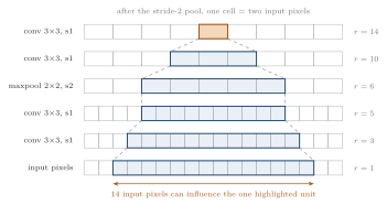
Stack: conv \(3{\times}3\) (s1) → conv \(3{\times}3\) (s1) → maxpool \(2{\times}2\) (s2) → conv \(3{\times}3\) (s1) → conv \(3{\times}3\) (s1). The stride products before each layer are \(1, 1, 1, 2, 2\), so \[ r \;=\; 1 + \underbrace{2\cdot 1}_{\text{conv}} + \underbrace{2\cdot 1}_{\text{conv}} + \underbrace{1\cdot 1}_{\text{pool}} + \underbrace{2\cdot 2}_{\text{conv}} + \underbrace{2\cdot 2}_{\text{conv}} \;=\; 14 . \] The two \(3{\times}3\) convs after the downsample contribute 4 pixels each; the same two convs before it would contribute 2 each. (Common error: forgetting that the pool contributes its own \((k-1) \cdot 1 = 1\) term.)
The same arithmetic, animated: the cone grows one board-sum term at a time, and the jump from \(+2\) to \(+4\) per conv right after the stride-2 pool is the moment the formula’s \(\prod_{i<l} s_i\) factor becomes visible:
Stride and pooling build a feature pyramid: early layers, small RF at high resolution (edges, textures); deep layers, large RF at low resolution (parts, objects). This hierarchy is the empirical signature of CNN features.
Architecture as prior
The frame to keep from this block: architecture is a prior about data. Convolution asserts locality and translation invariance and, where the assumption fits, buys three orders of magnitude in parameters. The general concept, building a symmetry into the map rather than hoping to learn it, is equivariance; one sentence today, returning in earnest for molecules and manifolds in the U6 seminars (Track C).
Why this matters later. The U-Net (U0.T4 / U0.L4) is exactly CNN inductive bias + multiscale processing: this section’s RF arithmetic is why its deep bottleneck sees the entire image, which a velocity field at low \(t\), where the input is nearly pure noise and only global structure exists, genuinely needs.
The recipe card
The session’s artifact, boxed and numbered. Later pre-plans and problem sets cite this box as “the U0.T2 defaults”; the slide version (slide-recipe-card) is re-shown in U0.L2 and referenced by the PS0 statement.
- Optimizer: AdamW, base learning rate \(3 \times 10^{-4}\), \(\beta = (0.9,\ 0.999)\), weight decay \(0.01\), with normalization parameters and embeddings excluded from decay.
- Schedule: linear warmup over 1–5% of total steps, then cosine decay to \(\approx 0\).
- Initialization: He (\(\operatorname{Var}[w] = 2/\text{fan}_{\text{in}}\)) for ReLU-family activations; zero-init the last layer where “output \(\approx 0\) at start” is sensible; velocity fields \(u_t^\theta\): yes.
- Normalization: GroupNorm (U-Nets) or LayerNorm (transformers) for generative nets; BatchNorm only in bootcamp classifiers.
- Batch size: the largest that fits in memory, and always reported.
Deviation from the card in any later lab is permitted in writing, with a reason. The point is not that these defaults are optimal everywhere, but that they are known-good for the models this course builds, and that unexplained optimizer drift stops being a confound in every experiment we run.
What’s next
Next session (U0.L2): the recipe card meets CIFAR-10: training a CNN properly, with schedules, MLflow logging, checkpointing, and seeding, all bolted onto the training-loop-template from U0.L1. One of the runs you will be handed has been deliberately sabotaged; you will diagnose it from the curves alone, using today’s pictures as the diagnostic charts.