U0.T2 — Making Training Work

Flow-Based Generative Models · UFRJ · 2026.2

01Same code, three seeds

The U0.L1 homework-lite, run properly

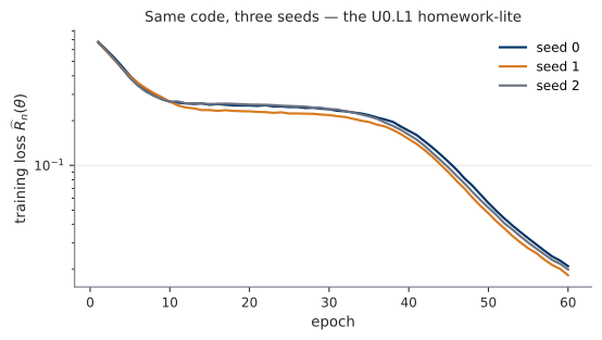
Same code, same data; only the seed changed. Today the variance is merely annoying. In a badly tuned run it decides whether training converges at all.

Question of the day: which settings (optimizer, schedule, initialization, normalization) make training reliably work, and what are our defaults?

Ask who ran the 3-seed homework-lite; show a student’s curves instead if any were sent in. The answer to the question of the day is literally the last slide: a recipe card the whole course will cite.

02Optimizers: SGD → momentum → Adam → AdamW

Gradient descent meets the minibatch

Full-batch GD on the empirical risk \(\widehat{R}_n(\theta)\) costs one pass over the dataset per step. Instead: sample a minibatch \(B \subset \{1,\dots,n\}\), step on its gradient.

The empirical measure of the minibatch, \(\widehat{q}_B = \frac{1}{|B|}\sum_{i\in B}\delta_{(x_i, y_i)}\), puts mass \(1/|B|\) on each sampled pair, so an expectation under it is simply the batch average: \[ \mathcal{L}_B(\theta) = \mathbb{E}_{(x,y)\sim \widehat{q}_B}\big[\ell\big(f_\theta(x),\,y\big)\big] = \frac{1}{|B|} \sum_{i \in B} \ell\big(f_\theta(x_i),\, y_i\big), \] and SGD iterates \(\theta_{k+1} = \theta_k - \eta_k\, g_k\), \(\;g = \nabla_\theta\, \mathcal{L}_B(\theta)\), with learning rate \(\eta_k\).

With \(B\) sampled uniformly, \(\;\mathbb{E}_{B}\big[g\big] = \nabla_\theta \widehat{R}_n(\theta)\): an unbiased estimator. Noisy, but pointing the right way on average.

Board 1 starts here and stays up through Block C: SGD update, then the moment recursions, then bias correction. Emphasize the subscripted expectation — even optimizer pseudocode carries sampling subscripts in this course. Say out loud: the empirical-measure notation is U0.T1’s \(\widehat{R}_n\) story specialized to a batch — \(\widehat{R}_n\) is the expectation under \(\widehat{q}_n\), the empirical measure of all \(n\) samples.

Noise scale vs. batch size

How noisy is \(g\)? Across random draws of \(B\) it scatters around its mean, and \(\operatorname{Cov}_B[g]\) measures that scatter. Averaging \(|B|\) independent per-sample gradients divides the covariance by \(|B|\): \[ \operatorname{Cov}_B\big[g\big] \;\approx\; \frac{1}{|B|}\, \Sigma(\theta), \qquad \Sigma(\theta) = \operatorname{Cov}_{(x,y)\sim \widehat{q}_n}\! \big[\nabla_\theta\, \ell\big(f_\theta(x), y\big)\big], \] with \(\Sigma(\theta)\) the covariance of a single sample’s gradient; the noise level shrinks like \(1/\sqrt{|B|}\).

• Small batch: noisy, cheap steps (some regularizing jitter). Large batch: cleaner steps, better hardware utilization, but not proportionally fewer steps.
• The noise never vanishes: every curve you saw on the first slide wiggles because of this term.

Practical rule (recipe card): batch size is chosen by memory, then reported.

The real enemy: ill-conditioning

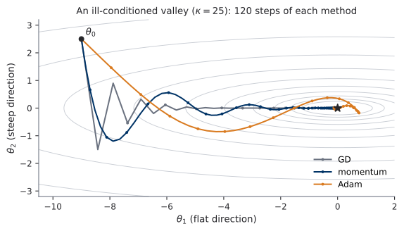
A valley, steep in \(\theta_2\) and flat in \(\theta_1\): GD’s single step size must be safe across the valley, hence agonizing along it. Real networks are far worse than \(\kappa = 25\).

Momentum: an EMA of gradients

Average the gradients instead of trusting the last one: \[ m_k = \beta\, m_{k-1} + (1-\beta)\, g_k, \qquad \theta_{k+1} = \theta_k - \eta\, m_k, \qquad \beta \approx 0.9 . \]

• \(m_k\) is an exponential moving average: oscillating components (across the valley) cancel; consistent components (along it) accumulate. That is the heavy-ball intuition: a ball with inertia rolling down the valley floor.
• PyTorch’s SGD(momentum=0.9) uses the un-normalized recursion \(m_k = \beta m_{k-1} + g_k\): same trajectory family, learning rate rescaled.
• Nesterov momentum: evaluate the gradient at the look-ahead point. Named so you recognize it; not derived.

Point back at the valley figure: blue curve = momentum damping the zigzag. The EMA form is chosen deliberately — Adam is two of these.

Adam: two EMAs and a per-coordinate step

\[ \begin{aligned} m_k &= \beta_1\, m_{k-1} + (1-\beta_1)\, g_k &&\text{(first moment: direction)}\\ v_k &= \beta_2\, v_{k-1} + (1-\beta_2)\, g_k^{\,2} &&\text{(second moment: scale)}\\ \widehat{m}_k &= \frac{m_k}{1-\beta_1^{\,k}}, \quad \widehat{v}_k = \frac{v_k}{1-\beta_2^{\,k}} &&\text{(bias correction: next slide)}\\ \theta_{k+1} &= \theta_k - \eta_k\, \frac{\widehat{m}_k}{\sqrt{\widehat{v}_k} + \varepsilon} &&\text{(defaults: } \beta_1 = 0.9,\ \beta_2 = 0.999,\ \varepsilon = 10^{-8}) \end{aligned} \]

Each coordinate gets its own effective step \(\eta_k / (\sqrt{\widehat{v}_k} + \varepsilon)\): coordinates with historically large gradients step small, and vice versa. That is the ill-conditioning fix, per coordinate and for free.

The race, animated

Same dynamics as the static figure (identical hyperparameters), plus what a curve cannot show: Adam’s per-coordinate state. Watch the two bars diverge — flat coordinate long, steep coordinate short — while the orange dot moves at a uniform rate. Slow phase = first 10 steps (GD’s alternation visible step by step); then time-lapse to 120.

Live derivation: the bias-correction factor

The EMAs start at \(m_0 = 0\), so early estimates are biased toward zero. Unroll, then take expectations, assuming the gradient distribution is roughly stationary over the window (\(\mathbb{E}_{B}[g_i] \approx g\)): \[ m_k = (1-\beta) \sum_{i=1}^{k} \beta^{\,k-i}\, g_i \quad\Longrightarrow\quad \mathbb{E}_{B}[m_k] \;\approx\; g\,(1-\beta)\sum_{i=1}^{k}\beta^{\,k-i} = g\,\big(1 - \beta^{\,k}\big). \] Dividing by \(1-\beta^{\,k}\) removes the startup bias; as \(k\) grows the correction retires. \(\square\)

Board 1, right column. Keep this visible: warmup (Block C) points straight back at \(\widehat{v}_k\) being untrustworthy for small \(k\).

AdamW: weight decay is not L2 when steps are adaptive

L2 regularization adds \(\frac{\lambda}{2}\lVert\theta\rVert_2^2\) to the loss; its gradient \(\lambda\theta\) shrinks every weight each step (“weight decay”). Under SGD the two views coincide. Under Adam they do not:

• L2 in the loss: \(\lambda\theta\) joins \(g_k\) and is divided by \(\sqrt{\widehat{v}_k}\): large-gradient coordinates are barely decayed, an accident of gradient history.
• Decoupled decay (AdamW): shrink the weights outside the adaptive machinery, \[ \theta_{k+1} = \theta_k - \eta_k \left( \frac{\widehat{m}_k}{\sqrt{\widehat{v}_k} + \varepsilon} \;+\; \lambda\, \theta_k \right), \] so every weight decays at the same rate \(\eta_k \lambda\), as intended.

The course optimizer is AdamW, with today’s recipe-card defaults, from U0.L2 through U3. Deviations must be justified in writing.

Honest empirics: what AdamW does not win

• On vision classification, well-tuned SGD + momentum often generalizes slightly better than Adam-family optimizers. That literature is real.
• Nobody trains large generative models that way: time-conditioned objectives with heterogeneous gradient scales across \(t\) are exactly the regime adaptive methods handle well.
• Our default is chosen for the models we build, not as a universal claim.

Every flow / CFM / DDPM lab in this course (U1.L1 … U3.L3) trains with AdamW under today’s defaults, and PS0 requires them. When a later loss \(\mathbb{E}_{t,\,x_1\sim q,\,x\sim p_t(\cdot\mid x_1)}[\cdots]\) mixes easy and hard time steps in one batch, the per-coordinate scaling is doing quiet work.

03Schedules: warmup + cosine

Why warmup exists

The bias-correction slide had a hidden warning: for small \(k\), \(\widehat{v}_k\) is an estimate built from a handful of samples.

• At step 10, the second-moment EMA has seen \(\sim 10\) gradients: \(\widehat{v}_k\) is garbage, and dividing by \(\sqrt{\text{garbage}}\) makes some coordinates take enormous steps.
• Early training is also where the loss surface is least friendly: the network is at a random init, gradients are large and unrepresentative.
• Large adaptive steps at random init destabilize runs that would otherwise be fine. The classic symptom is a loss spike (or NaN) in the first few hundred steps.

Fix: start the learning rate near zero and ramp it up linearly while the moment estimates fill up.

The course schedule, in one picture

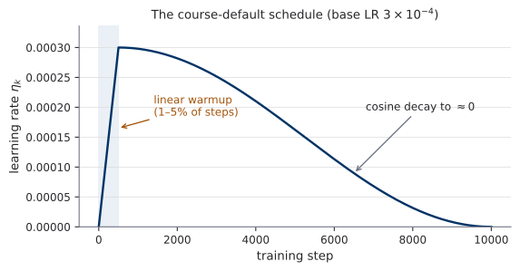
Terminology: a step is one optimizer update on one minibatch; an epoch is a full pass over the data, \(\approx n/|B|\) steps. Course schedules are defined per step.

Linear warmup over 1–5% of total steps, then cosine decay to \(\approx 0\). Anything else in a later lab must be justified in writing.

Point at Board 1: warmup is the operational answer to “when can I trust \(\widehat{v}_k\)?” Cosine: smooth, one parameter (total steps), ends near zero so late training polishes. Step vs epoch matters because U0.L2’s config file counts in steps. Mention: time-conditioned generative losses are noisy-gradient regimes; U3 labs assume this schedule silently.

04Initialization

The failure mode: exponential in depth

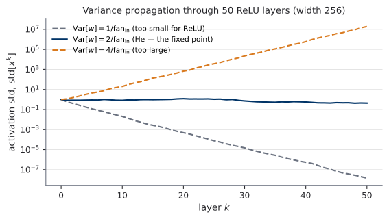
Depth multiplies scales: a per-layer factor \(c \ne 1\) becomes \(c^L\), geometric growth or death, inherited by the gradients through the backward pass. At depth 50, the wrong constant costs \(10^{7}\).

Live derivation: variance propagation

Setup: \(y = Wx\), entries of \(W\) i.i.d. with mean \(0\) and variance \(\sigma_w^2\), independent of \(x\), whose coordinates are i.i.d. with mean \(0\).

\[ \operatorname{Var}[y_i] = \sum_{j=1}^{d} \operatorname{Var}[w_{ij} x_j] = d\; \sigma_w^2 \operatorname{Var}[x] \qquad (d = \text{fan}_{\text{in}}). \] A ReLU halves the second moment of a symmetric input, \(\;\mathbb{E}\big[\operatorname{ReLU}(z)^2\big] = \tfrac{1}{2}\mathbb{E}[z^2]\), so one linear + ReLU layer maps \(\operatorname{Var}[x] \mapsto \tfrac{1}{2}\, d\, \sigma_w^2\, \operatorname{Var}[x]\); the scale is preserved iff \[ \sigma_w^2 = 2 / \text{fan}_{\text{in}} \qquad \textbf{(He initialization).} \]

Xavier/Glorot (\(\sigma_w^2 = 2/(\text{fan}_{\text{in}}+\text{fan}_{\text{out}})\)) is the tanh/linear analogue (no ReLU halving to undo). Stated, not derived.

Board 2: the chain Var → d σ² Var → ½ d σ² Var, then set the factor to 1. Keep visible into Block E — normalization is the other fix for the same disease. The ReLU halving: z symmetric ⇒ ReLU zeroes half the mass; one line if asked.

Initialization in practice

• Trust nothing by default. PyTorch’s nn.Linear init is not He: check what your framework does before assuming what a paper assumed. (You will verify this in U0.L2.)
• Zero-init the last layer when “output \(\approx 0\) at start” is sensible: the network begins as (near) the zero function, and training grows it from there.
  • For our velocity fields \(u_t^\theta\), small outputs at init mean early training is not fighting a random vector field. Standard practice from U3.L1 on.
  • The same idea returns, dressed up, as adaLN-zero in the DiT preview (U0.T4).

U0.L2’s sabotaged runs include a bad-init variant: you will be handed loss curves and asked to name the disease. Today’s figure (flat vs. dying vs. exploding scale) is the diagnostic chart.

05Normalization and residual connections

What normalization actually buys

Folklore first: BatchNorm was introduced (2015) to fix “internal covariate shift”, the story that layer-input distributions drifting during training is the core problem. The explanation did not survive; the method did.

What normalization demonstrably does:

• allows higher learning rates without divergence;
• reduces sensitivity to initialization (Board 2’s disease, treated at run time instead of init time);
• smooths the optimization landscape (empirically well documented; mechanism still debated).

Mechanism on the next slide; then the knife.

BatchNorm: mechanism and the train/eval split

\[ \mu_c = \mathbb{E}_{(x,y)\sim \widehat{q}_B}\big[x_c\big], \quad \sigma_c^2 = \operatorname{Var}_{(x,y)\sim \widehat{q}_B}\big[x_c\big], \quad \text{BN}(x_c) = \gamma_c\, \frac{x_c - \mu_c}{\sqrt{\sigma_c^2 + \varepsilon}} + \beta_c, \] with learned \(\gamma_c, \beta_c\); statistics taken over the batch and spatial positions.

• Train mode: normalize with the current batch’s statistics; keep running averages on the side.
• Eval mode: normalize with the running statistics. The model must work on a single sample.
• Two behaviors, one module: model.train() vs model.eval(). Forgetting the switch is a classic silent bug (U0.L2 will make you feel it).

The knife: batch statistics are a liability

Every sample’s output now depends on who else is in the batch:

• Small batches → noisy statistics → normalization itself injects noise (train/eval gap grows).
• Pointwise evaluation → there is no batch; running averages must faithfully stand in.
• Generative models condition on a per-sample time \(t\): a batch mixes samples at \(t \approx 0\) (pure noise) and \(t \approx 1\) (nearly data). Their activation statistics should differ; batch-normalizing across them couples what the model is trying to keep apart.

So the models we build need per-sample normalization. Two candidates, one picture →

LayerNorm and GroupNorm

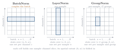
LN: per sample, all channels (transformers / DiT). GN: per sample, channel groups (U-Nets). Neither couples the batch; no train/eval split.

Generative models here use GroupNorm (U-Nets) or LayerNorm (transformers); BatchNorm only in this bootcamp’s CIFAR-10 classifier.

Residual connections

Deep stacks fail even when each layer is healthy: by depth 50, plain stacks are barely trainable. The fix is one plus sign: \[ x_{k+1} \;=\; x_k + f_k(x_k). \]

The gradient highway, in one line: the Jacobian \(\;\partial x_{k+1} / \partial x_k = I + \partial f_k / \partial x_k\;\) has an identity term, so the backward cotangent always has a direct path. Products of Jacobians no longer die like Board 2’s geometric chain, and depth stops being the enemy: this is what makes 50-block U-Nets and 30-block DiTs trainable.

Keep this innocuous plus sign in mind. In U1.T2 it becomes a theorem, and in U2 it becomes the whole course.

The gray line is a teaser, deliberately without a punchline — do NOT state any limit or continuous-time connection today; that reveal belongs to U1.T2’s cliffhanger. If someone pushes, smile and say “U1.T2”.

06CNNs and inductive bias

Convolution: a constrained linear map

A convolution layer is a linear map, with two constraints baked in:

1. Locality: each output looks at a \(k \times k\) window, not the whole image.
2. Weight sharing: the same window weights are used at every position, so shifting the input shifts the output: translation equivariance.

The striking number, CIFAR-10 sized (\(32 \times 32 \times 3 = 3072\) values):

Layer	Parameters
Fully connected, \(3072 \to 3072\)	\(\approx 9.4\)M
Conv \(3{\times}3\), \(3 \to 64\) channels	1,792

Three orders of magnitude fewer parameters, not by shrinking the model but by encoding an assumption about images. (Where 1,792 comes from: next slide.)

Anatomy of a convolution layer

• Kernel (filter): a \(k \times k \times C_{\text{in}}\) block of weights. Sliding it over the input and taking a dot product at each position produces one feature map; a layer with \(C_{\text{out}}\) kernels outputs \(C_{\text{out}}\) channels.
• Stride \(s\): the window moves \(s\) pixels at a time; \(s > 1\) downsamples the output by a factor of \(s\).
• Padding: zeros added around the border so windows fit at the edges; “same” padding keeps the spatial size unchanged.
• Pooling: parameter-free downsampling: take the max (or mean) over each window, typically \(2{\times}2\) with stride 2, halving the resolution.

Parameter count: \(\;k \cdot k \cdot C_{\text{in}} \cdot C_{\text{out}} + C_{\text{out}}\;\) (one bias per output channel). The table’s conv layer: \(3 \cdot 3 \cdot 3 \cdot 64 + 64 = 1{,}792\).

This is deliberately a vocabulary slide — students arrive with wildly uneven CNN exposure. The four terms here are exactly the ones the U0.L2 CNN and the U0.L4 U-Net configs use.

Receptive fields

The receptive field of a unit: the input region that can influence it. Strides multiply how fast it widens.

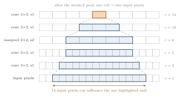
\[ r_L \;=\; 1 + \sum_{l=1}^{L} (k_l - 1) \prod_{i=1}^{l-1} s_i \qquad (k_l, s_l = \text{kernel size, stride of layer } l). \]

Receptive fields: the board arithmetic

Stack: conv \(3{\times}3\) → conv \(3{\times}3\) → maxpool \(2{\times}2\) stride 2 → conv \(3{\times}3\) → conv \(3{\times}3\). Stride products before each layer: \(1, 1, 1, 2, 2\), so \[ r = 1 + 2 + 2 + 1\cdot 1 + 2\cdot 2 + 2\cdot 2 = 14 . \] Two cheap \(3{\times}3\) convs after a downsample buy what one expensive \(9{\times}9\) would before it: striding is how deep layers get to see the whole image.

Note the pool’s own term: kernel 2, stride product 1 before it, so it contributes \((2-1)\cdot 1 = 1\).

Board 3: run the sum term by term against the diagram (previous slide): r = 1, 3, 5, 6, 10, 14 row by row. Common student error: dropping the pool’s own +1 term — it is called out on the slide now.

The cone, animated

The cone grows bottom-up, one board-sum term at a time; the counter and the formula tick together. The beat to narrate: after the stride-2 pool, the two convs add 4 pixels each instead of 2 — the ×2 magnification the formula’s stride product encodes.

Feature hierarchies, and architecture as prior

• Stride/pooling builds a pyramid: early layers see edges (small RF, high resolution); deep layers see objects (large RF, low resolution). This hierarchy is the empirical signature of CNN features.
• The frame to keep: architecture = prior about data. Convolution asserts “statistics are translation-invariant and local”; when the assumption fits, you pay thousands of parameters instead of millions.
• The general concept is equivariance: build the symmetry into the map rather than learning it. One sentence today; it returns in U6 (Track C).

The U-Net (U0.T4 / U0.L4) is exactly CNN inductive bias + multiscale processing: today’s RF arithmetic is why its deep bottleneck sees the whole image, which a velocity field at low \(t\) genuinely needs.

07The recipe card

The course training defaults

1. Optimizer: AdamW, base LR \(3 \times 10^{-4}\), \(\beta = (0.9,\, 0.999)\), weight decay \(0.01\), excluding normalization parameters and embeddings from decay.
2. Schedule: linear warmup over 1–5% of total steps, then cosine decay to \(\approx 0\).
3. Init: He for ReLU-family activations; zero-init the last layer where “output \(\approx 0\) at start” is sensible (velocity fields \(u_t^\theta\): yes).
4. Normalization: GroupNorm (U-Nets) / LayerNorm (transformers) for generative nets; BatchNorm only in bootcamp classifiers.
5. Batch size: the largest that fits in memory, and always reported.

Say aloud: deviating from the card in a later lab is allowed — in writing, with a reason. Kept off the slide so the card stays the full-height named asset it is (the AdamW slide already states the same rule in its box).

Close: next session (U0.L2)

• Next session (U0.L2): this recipe meets CIFAR-10 for real. Schedules, logging (MLflow), checkpointing, seeding.
• One of the runs you will be given has been sabotaged. You will diagnose it from the curves alone; today’s pictures are the diagnostic charts.

See you next session.