U0.L2 — Training Hygiene on CIFAR-10
Session U0.L2 · date: see calendar-map
This lab upgrades the U0.L1 training-loop-template into the hygiene stack — template v2: config-driven runs, experiment tracking with MLflow, learning-rate schedules and checkpoint discipline per the U0.T2 recipe card, and reproducibility as a recorded, checkable property rather than a hope. The stack is frozen at the end of the session and never re-taught; every later lab assumes it, and the PS0 problem statement requires — verbatim — that your models were “trained with the hygiene stack.” After today, that phrase names a specific artifact and the claim is checkable: config, seed, commit, and MLflow store in the submission.
The session has a second job, equally important. Its centerpiece is the mystery run: you will be handed a training run that has been deliberately sabotaged, and you must diagnose it from its logged curves alone — the configs are scrubbed. This is deliberate training for the main course. A CIFAR-10 classifier is the last model in this course you can debug by eyeballing its outputs; you cannot look at a velocity field \(u_t^\theta\) and see the bug. You can read its loss curve, its gradient norms, its throughput — and the whole point of today’s logging discipline is that the curves speak the same language no matter how strange the model gets.
Format shift, deliberate. U0.L1 was a notebook; today is scripts and a terminal: train_cifar.py, launched with a config file. Hygiene is about runs — things you launch, tag, compare, and resume — and a run is a terminal artifact, not a cell you re-execute. Notebooks return for the exploratory labs (U0.L3 onward), where the object of study is code you are still shaping; today the object of study is the run itself.
Compute reality. CIFAR-10 in a 90-minute lab means short runs — 5–8 epochs of a small ResNet. Curves, not accuracy, are the object of study; the instructor’s precomputed 30-epoch reference run ships alongside the lab for comparison overlays.
Standing reference for the training mechanics touched today: Bishop and Bishop (Bishop and Bishop 2024). The optimizer, schedule, initialization, and normalization reasoning behind every default used here is the previous theory session (U0.T2) — cited below as the recipe card, never re-derived.
A · From template to stack
Reused in: every later lab and PS0 — this is how all course experiments launch.
The repo layout from U0.L1 grows by two directories:
your-course-repo/
  labs/       # notebooks — exploratory labs return in U0.L3
  common/     # train.py: template v1 now, v2 by the end of today
  configs/    # NEW: one yaml per run
  runs/       # checkpoints (gitignored)
  mlflow.db   # NEW: MLflow store (sqlite, gitignored)
One run = one config = one MLflow run
The first hygiene rule is that an experiment is data, not code. Every quantity that can vary between runs — architecture, optimizer settings, schedule, seed, data options, the run’s own name — lives in a config file; the code reads the config and contains no magic numbers.
run_name: U0L2-baseline-s0
seed: 0
data:  {root: ./data, dataset: cifar10, normalize: true, batch_size: 256}
model: {arch: resnet9, norm: batch}      # classifier => BN allowed (U0.T2 law)
opt:   {name: adamw, lr: 3.0e-4, betas: [0.9, 0.999], weight_decay: 0.01}
sched: {name: warmup_cosine, warmup_frac: 0.03}
epochs: 8
The payoff is comparability: two runs differ by a config diff — a small, inspectable object — never by an edit history you have to reconstruct from memory. When a result surprises you in week 10, diff configs/a.yaml configs/b.yaml answers “what changed” in one second.
TODO A.1 (config part). Wire the config into the U0.L1 Trainer without breaking its interface. The loader is small — yaml.safe_load into a dataclass — and a build(cfg) factory constructs the model, optimizer, and scheduler from it. The v2 Trainer adds only keyword-only optional arguments (sched=None, tracker=None), so every v1 call site — including your U0.L1 notebook — still runs. This is the contract discipline you will meet in every well-maintained library: extend in place, preserve the interface.
B · Experiment tracking with MLflow
Reused in: everything — the U3.L1 payoff plot is an MLflow run comparison across sessions.
The standing decision
The course logging standard is MLflow, deployed locally: the UI runs on your own machine (mlflow ui --backend-store-uri sqlite:///mlflow.db), backed by a local SQLite file next to your code (run artifacts land in mlartifacts/). The criteria, on the record:
- open source, zero vendor accounts — nothing to sign up for, nothing that expires mid-semester;
- data sovereignty — your runs stay on your machine, fully offline by construction;
- production alignment — of the trackers you may meet at work, MLflow is the most likely;
- run comparison built in — the within-experiment overlay view is exactly the instrument the mystery run (today) and the U3.L1 simulation-free-vs-simulation-based payoff plot (later) require.
You may meet wandb or TensorBoard elsewhere; the concepts transfer one-for-one and we name them once here, without teaching them. You may also meet the mlruns/ file-store backend in older MLflow tutorials — it is deprecated as of MLflow 3.15 (it raises unless you opt out via an environment variable), which is why the course standardizes on the SQLite backend MLflow itself recommends. The mlflow package is pinned in the course lockfile (3.15.1).
Wiring the Trainer
import mlflow

mlflow.set_tracking_uri("sqlite:///mlflow.db")
mlflow.set_experiment("fbgm-2026")            # ONE experiment per course phase

with mlflow.start_run(run_name=cfg.run_name):
    mlflow.log_params(flatten(cfg))           # the resolved config, at start
    mlflow.set_tags({"session": "U0.L2", "tag": "baseline", "seed": cfg.seed})
    trainer.fit(train_loader, val_loader, epochs=cfg.epochs)
Note what is logged when: the resolved config (after defaults and overrides are merged) is logged as params at run start, so the record reflects what actually ran, not what the template intended. Inside fit, the v2 template logs at two cadences — per step: train loss and learning rate; per epoch: val loss and accuracy, gradient norm (global \(L_2\)), weight norm, and throughput (images/second).
TODO B.1 (tracking part). Add the mlflow.log_metric calls to your v2 fit at exactly these two cadences.
What to log, and why
This checklist is one half of the hygiene-stack artifact. Each line is a sensor; the mystery run below is the exercise in reading them.
- Train AND val loss — the gap between them is the first diagnostic of overfitting and of data bugs.
- Learning rate — schedule bugs are the #1 silent killer. Log what the optimizer actually used (from its param group), not what the config asked for: the whole point is catching divergence between intent and execution.
- Gradient norm (global \(L_2\)) — explosions and vanishing, visible live. U0.T2’s variance-propagation pictures are what make these curves readable.
- Weight norm — weight-decay and initialization sanity.
- Throughput (img/s) — a sudden drop is the silent-CPU-fallback detector, and the first hint of a dataloader bottleneck.
- Sample/prediction figures via
mlflow.log_figure— today a grid of misclassified images; in U3, the same call logs generated-image panels. This is the workflow for qualitative tracking from here to the end of the course.
The live demonstration in the lab: launch two short baseline runs with seeds 0 and 1, open mlflow ui, select both, and read the compare view. The loss curves wiggle differently and land together — that spread is the seed variance you eyeballed in the U0.L1 homework-lite, now measured. The LR curves are identical — the schedule is deterministic. And the params differ in exactly one field: seed. Config diff = run diff.
C · Schedules and checkpoints
The recipe card becomes running code
Every default in this lab comes from the U0.T2 defaults — the recipe card (optimizer-schedule-defaults) boxed at the end of the U0.T2 notes: AdamW at base LR \(3\times 10^{-4}\), \(\beta = (0.9, 0.999)\), weight decay \(0.01\) with normalization parameters and embeddings excluded; linear warmup over 1–5% of steps then cosine decay to \(\approx 0\); He initialization for ReLU-family activations; and — the one clause that is ours today — BatchNorm only in bootcamp classifiers, which is exactly what a CIFAR-10 ResNet is. We cite the card; we do not re-derive it.
The schedule wires in as a step-wise multiplier on the base LR:
def warmup_cosine(step: int) -> float:          # multiplier on base LR
    if step < warmup_steps:
        return step / max(1, warmup_steps)
    p = (step - warmup_steps) / max(1, total_steps - warmup_steps)
    return 0.5 * (1.0 + math.cos(math.pi * p))

sched = torch.optim.lr_scheduler.LambdaLR(opt, warmup_cosine)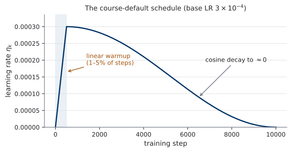
TODO C.1 (schedule part). Add sched to the v2 Trainer — stepped per step, not per epoch — and confirm in the MLflow UI that the logged learning rate traces Figure 1. The plot is the test: this is the instrument-then-verify habit the whole session installs. (The classic failure — a flat LR curve — means you stepped the scheduler per epoch.)
Checkpoint discipline
Two files per run, updated on different triggers:
last.pt— saved every epoch, unconditionally. This is the resume point.best.pt— saved only when the validation metric improves. This is the deliverable. Selection is on val, by a named metric, never on test.
{"model":  model.state_dict(),   "opt":   opt.state_dict(),
 "sched":  sched.state_dict(),   "epoch": epoch,
 "config": cfg,                  "mlflow_run_id": run_id}
A checkpoint that cannot resume is just a weights file. Hence the optimizer state (Adam’s moment estimates are state you cannot reconstruct), the scheduler state (or your LR restarts from warmup), the epoch counter, the config that produced the run, and the MLflow run id that ties the file on disk back to its curves.
TODO C.2 (checkpoint part). Implement resume-from-checkpoint in the v2 Trainer, then prove it with the round-trip assert: train one epoch → save → load into a fresh Trainer → evaluate → assert the val loss is identical (tolerance \(10^{-6}\); fixed seed, same machine). Why we are strict now: in U3 your models cross session boundaries — U3.L2’s trained flow is reused in U3.L3 for classifier-free guidance. A resume bug discovered there costs a lab session; discovered here it costs five minutes. The usual suspects when the round trip does break: BatchNorm running statistics saved while the model was in train mode; a scheduler that was never saved; the scheduler constructed after the optimizer state was loaded (scheduler construction runs step 0 and overwrites the restored learning rate — your first resumed batch silently trains at the warmup LR of zero); or an in-memory “checkpoint” holding state_dict() references rather than copies, so later training mutates it in place (torch.save serializes copies, which is why the bug only bites in-process).
The full-restore-vs-weights-only story is animated below: the same run checkpointed and killed, then resumed both ways. The full restore traces the uninterrupted run exactly — bit-equal, asserted in the generating script. The weights-only restore is a different run wearing your weights: the learning rate restarts onto fresh Adam moments and the loss spikes. Watch the honest ending, too — on this toy the fork recovers. The lesson is not “weights-only trains worse”; it is that you are no longer training the run you think you are.
D · Reproducibility
Seeds, completely this time
set_seed(seed) from U0.L1 seeds Python, NumPy, and torch (including CUDA). Two gaps remain, and both live in the dataloader:
loader = DataLoader(ds, batch_size=cfg.data.batch_size, shuffle=True,
                    generator=torch.Generator().manual_seed(cfg.seed),
                    worker_init_fn=seed_worker)   # workers get derived seeds
Without the explicit generator, the shuffle order depends on global RNG state; without worker_init_fn, each worker process seeds itself independently of your seed — so the same config with num_workers: 0 and num_workers: 4 produces different batch orders. Reproducibility that depends on a performance setting is not reproducibility.
Full bitwise determinism exists — torch.use_deterministic_algorithms(True) — and comes with an honest caveat: it costs speed, and some GPU ops simply have no deterministic implementation. The course policy: deterministic for debugging, fast for training, always seeded.
Capture the environment
A run you cannot reconstruct is a run you cannot defend. Three captures, all cheap:
Environment:
pip freeze > requirements.lock, committed per lab.Code version: the git commit hash, logged as an MLflow tag:
mlflow.set_tag("git_commit",
    subprocess.check_output(["git", "rev-parse", "HEAD"]).decode().strip())
Data version: the dataset name and version pinned in the config (
dataset: cifar10— torchvision’s copy is versioned by the package pin in the lockfile).
MLflow does auto-capture the commit — a mlflow.source.git.commit tag (plus branch and repo URL) appears whenever a script file is launched from inside a repository; we verified this with the lab’s own launcher. Two lessons ride on that sentence. First, verification has teeth only when it uses the artifact you actually ship: our first check ran code via python -c, which has no source file for MLflow to inspect, and concluded the opposite. Second, the auto-record has a hole — it carries no dirty flag. Launch with uncommitted edits and the auto-tag records the same clean-looking SHA; a commit hash from a dirty tree is a lie, because the code that ran is not the code the hash names. TODO D.1 (repro part): find mlflow.source.git.commit among your run’s tags in the UI and confirm it matches git rev-parse HEAD. Now look for any dirty indicator next to it — there is none. That is why the template logs git_commit and git_dirty itself, unconditionally: your provenance record should not depend on tracker internals, and it must say when the hash cannot be trusted. A dirty working tree deserves special suspicion: a commit hash logged from a dirty tree is a lie, because the code that ran is not the code the hash names.
- Seed — set once, logged as a param, dataloader workers included.
- Config — the resolved config logged at run start; no magic numbers in code.
- Commit — git hash as a tag; dirty tree means the hash is a lie.
- Environment — lockfile committed alongside the lab.
- Data version — dataset name + version pinned in the config.
Five lines, and none of them is aspirational: PS0 is graded on correctness and reproducibility — this checklist, not sample quality, is the rubric.
E · The mystery run
One of the runs you are about to load has been deliberately sabotaged. Nobody will tell you how.
Setup
unzip mystery-runs.zip
mlflow ui --backend-store-uri sqlite:///mystery.db
The export contains the sabotaged runs and clean baselines (three seeds each), plus the instructor’s 30-epoch reference run. It is fully offline, requires no accounts, and is identical for everyone.
Rules of engagement. The logged params and tags of the sabotaged runs have been scrubbed — you cannot read the bug off a config field. Curves and metrics only. Everything you need was covered in the previous sixty minutes.
The task
From curves alone, in pairs:
- Describe the pathology — what is wrong, in observable terms?
- Name at least two candidate causes.
- Rank them — which is more likely, given these curves?
- Propose the single cheapest discriminating experiment — the one measurement that best separates your top candidates.
- Run it. Confirm or kill your hypothesis.
Steps 3–4 are the discipline this exercise trains: not “what could be wrong” — everything could be wrong — but “what would you look at first, and why.” A bare “it’s the data” scores zero without the ranking and the discriminating experiment; the five steps are the deliverable, not the bug’s name.
What a discriminating experiment looks like here: log the input batch statistics (mean/std) of the training data; overlay per-layer gradient or weight norms, mystery vs. clean; rerun 20 steps at a lower learning rate and see whether the pathology moves. Each costs minutes — and that is the point. The cheapest test that splits your top two hypotheses is almost always this cheap; the expensive habit it replaces is re-running the whole thing with changes made on a hunch.
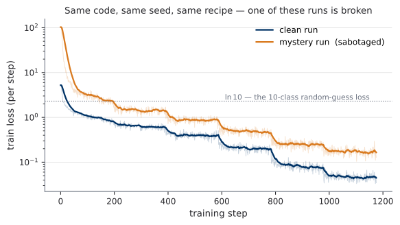
The 30 minutes run in three phases: ten minutes of silent curve-reading in pairs; ten minutes of board round — hypotheses collected, forced ranking, “what would you look at first and why”; ten minutes to run the discriminating experiment and the reveal. Fast finishers get a second sabotaged run (a different pathology, same five-step task).
The bug: bad initialization. The sabotaged run’s final linear layer — the classifier head — had its weights scaled ×20 at initialization, a one-line corruption of the init the recipe card prescribes. (Zero-init of last layers, the card’s clause 3, exists precisely to make this class of accident impossible.)
The signature, and how each logged sensor reports it (all numbers from the instructor’s prep runs — same seed, same recipe, 6 epochs). The initial loss opens at ≈ 97 against the clean run’s ≈ 4.9 — a factor of 20, the planted scale itself, and forty times above \(\ln 10 \approx 2.30\), the 10-class random-guess loss. An untrained network should be ignorant, not confidently wrong: an opening loss far above the random-guess line means the logits are enormous before any learning has happened, which points at scale — of the inputs, of the initialization — rather than at data or schedule. The descent then runs parallel to the clean curve but never closes the gap; at equal steps the sabotaged run lands at 69.8% val accuracy against 84.5% — the recipe’s warmup–cosine budget was spent undoing the sabotage.
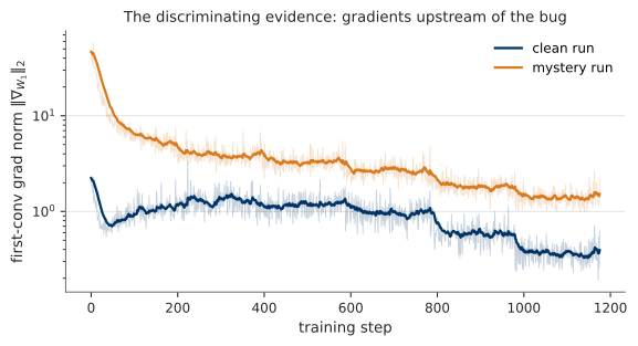
Where the evidence concentrates — an inversion worth remembering. The head’s own gradient norm barely separates (×1.5): its gradient is (logit error) × (pooled features), and the saturated softmax bounds the error factor. But every gradient flowing back through the ×20 weights is multiplied by 20 on the way down — so the first conv, the layer farthest from the sabotage, shows a ×21 gradient-norm gap. The bug is in the head; the smoking gun is in layer 1. Meanwhile the per-epoch weight norm (checklist item 4) reports the sabotage directly: the head’s weight norm starts twenty times too large. Two independent sensors, both on the Block B checklist, both decisive.
The full mechanism — why one scale bug vanished and the other fired — is animated below: per-layer activation and gradient meters, measured at initialization (every number on screen is real, from the seeded prep runs). Watch the first BatchNorm clamp the ×132 input spike back to std 1.000 in a single layer, then watch the head bug’s gradients blow up everywhere except the layer that contains the bug.
The bug we tried first — a negative result worth more than the exercise. The classic candidate — feeding raw \([0,255]\) pixels instead of standardized inputs — was planted first, and produced no signature at all: initial loss 4.91 vs 4.93, first-conv grad norms 0.95 vs 0.95, final accuracy 84.5% vs 84.6%. On this architecture the textbook bug is a non-event: BatchNorm absorbs the input scale in the forward pass, its backward pass symmetrically rescales the gradients, and AdamW’s per-parameter normalization mops up the rest. The “normalize your inputs” lore predates normalization-everywhere architectures. The meta-lesson pairs with the bug that did fire: a scale bug is diagnosable exactly when no normalization layer stands between it and the loss — the head is the one place BatchNorm cannot save you. (And the prep-side lesson, which is this course’s whole method: verify your planted bugs — and your intuitions — empirically.)
Why this bug was chosen. It is diagnosable purely from the logged curve set, given the initialization/scale reasoning of U0.T2 Blocks B–D; and it rewards precisely the sensors that Block B’s checklist made you log — vindicating, forty minutes later, the claim that every line of that checklist earns its place.
The lesson, verbatim from the session close:
You debugged a model without reading its config. In U2 and U3 the models get stranger, but the curves speak the same language. Log first, hypothesize second, discriminate cheaply third.
F · The clean baseline, and the freeze
The session closes by putting everything together once, live: launch the clean CIFAR-10 baseline with the full stack —
python train_cifar.py --config configs/baseline.yaml— and, in the compare view, overlay your live run against the 30-epoch reference that shipped inside mystery-runs.zip. Your curve should trace the reference’s early epochs; if it does not, you now own the diagnostic toolkit to say why. (If your throughput curve is suspiciously low, you have just met the silent-CPU-fallback detector in person.)
hygiene-stack = training-loop-template v2 (config-driven + MLflow tracking + schedules + checkpoint discipline) + the what-to-log checklist + the reproducibility checklist.
Commit it. This exact code trains every model you build in this course — the flows of U1, the CNFs of U2, the flow-matching models of U3 — and PS0’s requirement “trained with the hygiene stack” refers to this artifact by name. Deviations in later labs are permitted the same way deviations from the recipe card are: in writing, with a reason.
Next session (U0.T3): we go latent. Latent-variable models, the ELBO, and the variational autoencoder — the first models of this course that generate. The hygiene stack is assumed from here on, never re-taught, always required. Your CIFAR-10 baseline keeps training tonight; look at its curves tomorrow — you know how now.