U0.L2 — Training Hygiene on CIFAR-10

Flow-Based Generative Models · UFRJ · 2026.2

01From template to stack

Today your training loop grows up

By the end of these 90 minutes, the U0.L1 training-loop-template becomes the hygiene stack — template v2:

• config-driven runs — no magic numbers anywhere,
• experiment tracking (MLflow) — every run logged, comparable, permanent,
• schedules + checkpoint discipline — the U0.T2 recipe card, wired in,
• reproducibility — seed, config, commit, environment: all recorded.

The stack is frozen today and never re-taught. PS0 will require, verbatim: “trained with the hygiene stack” — after today that is a checkable claim.

Centerpiece (30 min): the mystery run — one of the runs you will be handed has been sabotaged. You will diagnose it from its curves alone.

One minute, then move. The mystery-run announcement up front changes how they listen to B–D: every logged quantity becomes a future diagnostic instrument. Say it exactly that way — “everything we log in the next hour is a sensor you will need at minute 50.”

Why this lab is scripts, not a notebook

Hygiene is about runs — things you launch, tag, compare, and resume. A run is a terminal artifact, not a cell you re-execute:

python train_cifar.py --config configs/baseline.yaml

Two new top-level directories in the course repo layout:

your-course-repo/
  labs/       # notebooks return in U0.L3
  common/     # train.py: v1 now, v2 today
  configs/    # NEW: one yaml per run
  runs/       # checkpoints (gitignored)
  mlflow.db   # NEW: MLflow store (sqlite, gitignored)

Notebooks are for studying code; scripts are for studying runs. Today’s object of study is the run.

One run = one config = one MLflow run

run_name: U0L2-baseline-s0
seed: 0
data:  {dataset: cifar10, normalize: true, batch: 256}
model: {arch: resnet9, norm: batch}  # classifier: BN ok
opt:   {name: adamw, lr: 3.0e-4, weight_decay: 0.01}
sched: {name: warmup_cosine, warmup_frac: 0.03}
epochs: 8

No magic numbers in code — anything that can vary between runs lives here; two runs differ by a config diff, never an edit history.

TODO A.1 (config part): wire the config into the U0.L1 Trainer — interface preserved (v2 adds only keyword-only optional args).

Reused in: every later lab and PS0 — this is how all course experiments launch; say so. Live-code the loader (yaml.safe_load → a small dataclass) and the build(cfg) factory. Emphasize the contract: the U0.L1 interface is preserved — this is how real libraries evolve. Point at normalize: true without comment; it earns its keep later.

02Experiment tracking with MLflow

The standing decision: MLflow, running locally

The course logging standard, fixed today and used through U3:

• Open source, zero vendor accounts — nothing to sign up for,
• your data stays on your machine — a local SQLite file, fully offline,
• production alignment — the tracker you are most likely to meet at work,
• run comparison built in — the overlay view is exactly what the mystery run (today) and the U3.L1 payoff plot (later) need.

mlflow ui --backend-store-uri sqlite:///mlflow.db

You may meet wandb or TensorBoard elsewhere — same concepts, different plumbing. We name them once and move on.

The rationale is on the record in the course notes; don’t linger. If someone asks “why not wandb”: accounts + data leaves the machine — both disqualifying for a course setting.

Wiring the Trainer

Reused in: every training run for the rest of the course.

import mlflow
mlflow.set_tracking_uri("sqlite:///mlflow.db")
mlflow.set_experiment("fbgm-2026")  # ONE per course phase

with mlflow.start_run(run_name=cfg.run_name):
    mlflow.log_params(flatten(cfg))  # resolved config
    mlflow.set_tags({"session": "U0.L2",
                     "tag": "baseline", "seed": cfg.seed})
    trainer.fit(train_loader, val_loader, cfg.epochs)

TODO B.1 (tracking part): add the mlflow.log_metric calls inside fit — per step: train loss, lr; per epoch: val loss/acc, grad norm (global \(L_2\)), weight norm, throughput (img/s).

Naming and tags — conventions that scale to U3

One experiment per course phase; tags do the filtering.

Convention	Value
Experiment	fbgm-2026
Tags	session = U0.L2 · tag = baseline · seed = 0
Run name	{session}-{tag}-s{seed} → U0L2-baseline-s0

Why tags and not one experiment per session: cross-session overlays. In U3.L1 you will overlay your U2.L2 (simulation-based) runs against your U3.L1 (simulation-free) runs — same experiment, filtered by session tag. That plot is the punchline of the whole course arc; the convention that makes it possible costs nothing today.

This is the one place where a boring convention has a dramatic payoff — flag it. Students who invent their own naming schemes today will pay in U3.

What to log, and why

This checklist is one half of the hygiene-stack artifact.

1. Train AND val loss — the gap between them is the first diagnostic.
2. Learning rate — schedule bugs are the #1 silent killer; log what the optimizer actually used, not what the config asked for.
3. Grad norm (global \(L_2\)) — explosions and vanishing, visible live; U0.T2’s init/scale pictures made these curves readable.
4. Weight norm — decay and init sanity.
5. Throughput (img/s) — a sudden drop is the silent-CPU-fallback detector.
6. Sample/prediction figures via mlflow.log_figure — in U3 this same call logs generated-image panels.

5-minute mini-lecture. Say it out loud: every line earns its place at minute 50 — you diagnose ONLY what you logged. Point 2’s phrasing matters: log the LR from the optimizer’s param group, not from the config — the whole point is catching divergence between intent and execution.

Live: two seeds in the compare view

Launch two short baseline runs, seeds 0 and 1, then:

mlflow ui        # select both runs -> Compare

What you should see, and say out loud:

• the two loss curves wiggle differently but land together — that spread is the seed variance you eyeballed in the U0.L1 homework-lite, now measured;
• the LR curves are identical — the schedule is deterministic;
• params differ in exactly one field: seed. Config diff = run diff.

This is the demo beat — 5 minutes, everyone runs it. The three bullets are the guided-looking script; the compare view is the tool they will use unsupervised in Block E. CPU fallback is fine here: 1–2 epochs is enough to see curves.

03Schedules and checkpoints

The recipe card, back on screen

Cited from the previous theory session, not re-derived — this box is the U0.T2 defaults:

1. Optimizer: AdamW, base LR \(3 \times 10^{-4}\), \(\beta = (0.9,\ 0.999)\), weight decay \(0.01\); norm parameters and embeddings excluded from decay.
2. Schedule: linear warmup over 1–5% of steps, then cosine decay to \(\approx 0\).
3. Initialization: He for ReLU-family; zero-init last layers where sensible.
4. Normalization: GN/LN for generative nets; BatchNorm only in bootcamp classifiers — that is us, today, deliberately.
5. Batch size: largest that fits; always reported.

Today the card stops being advice and becomes running code.

Wiring warmup–cosine

def warmup_cosine(step):        # multiplier on base LR
    if step < warmup:
        return step / warmup
    p = (step - warmup) / (total - warmup)
    return 0.5 * (1 + math.cos(math.pi * p))

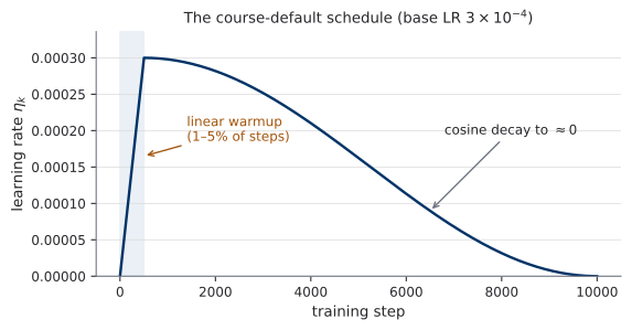
TODO C.1 (schedule part): wrap in LambdaLR, step per step, and check the logged LR traces this curve. The plot is the test.

“The plot is the test” is the habit being installed: instrument-then-verify beats trust. Anyone whose LR curve is flat stepped the scheduler per epoch.

Checkpoint discipline: last.pt and best.pt

Two files per run, updated on different triggers:

• last.pt — every epoch, unconditionally: the resume point.
• best.pt — only when the val metric improves: the deliverable. Selection is on val, by a named metric — never on test.

{"model": model.state_dict(), "opt": opt.state_dict(),
 "sched": sched.state_dict(), "epoch": epoch,
 "config": cfg, "mlflow_run_id": run_id}

A checkpoint that cannot resume is just a weights file — hence the optimizer/scheduler state and the config.

Resume must actually work

TODO C.2 (checkpoint part): implement resume-from-checkpoint in the v2 Trainer, then prove it with the round-trip assert:

# train 1 epoch -> save -> load into a fresh Trainer
# -> evaluate: the val loss must come back identical
assert abs(val_before - val_after) < 1e-6

Why we are strict now: in U3 your models cross session boundaries — U3.L2’s trained flow is reused in U3.L3 for classifier-free guidance. A resume bug discovered there costs a lab; discovered here it costs five minutes.

The bad resume, animated

The same two-moons run, checkpointed at epoch 20 of 30 (precomputed, seeded, CPU-deterministic). Beats: run + save_ckpt card → process killed → full restore traces the ghost EXACTLY (round-trip assert; bit-equal continuation) → weights-only restore forks: LR restarts onto fresh Adam moments, transient spikes. Deliver the honest ending out loud: on this toy the fork RECOVERS — the point is not “worse”, it is “a different run wearing your weights”; at U3 scale that costs you the run.

The 1e-6 tolerance is the fixed-seed same-machine case (course tolerance table). If someone hits a real mismatch: usual suspects are BN running stats saved in train mode, or the scheduler not saved. Both are worth saying out loud when they happen — they are the lab’s best organic teaching moments.

04Reproducibility

Seeds, again — now with dataloaders

set_seed(cfg.seed) from U0.L1 covers python / NumPy / torch / CUDA. Two gaps it does not cover:

loader = DataLoader(
    ds, batch_size=cfg.data.batch_size, shuffle=True,
    generator=torch.Generator().manual_seed(cfg.seed),
    worker_init_fn=seed_worker)  # workers: derived seeds

• Without these, shuffling order changes with worker count.
• Full determinism exists: torch.use_deterministic_algorithms(True) — honest caveat: slower, and some GPU ops are simply unsupported.

Course policy, verbatim: deterministic for debugging, fast for training, always seeded.

Demo the failure if time allows: same seed, num_workers 0 vs 4, different batch order. The policy line is the takeaway; it recurs in every later lab.

Capture the environment

A run you cannot reconstruct is a run you cannot defend. Three captures, all cheap:

• Environment: pip freeze > requirements.lock — committed per lab.

• Code version: the git commit, as an MLflow tag:

  sha = subprocess.check_output(
      ["git", "rev-parse", "HEAD"]).decode().strip()
  mlflow.set_tag("git_commit", sha)

• MLflow auto-captures the commit for script runs (verified) — but records no dirty flag: on a dirty tree the auto-SHA is a lie.

TODO D.1 (repro part): find mlflow.source.git.commit in your tags; now look for a dirty flag — none. Hence our own git_commit + git_dirty.

The reproducibility checklist

The other half of the hygiene-stack artifact.

1. Seed — set once, logged as a param, workers included.
2. Config — the resolved config logged at run start; no magic numbers.
3. Commit — git hash as a tag; dirty tree means the hash is a lie.
4. Environment — lockfile committed alongside the lab.
5. Data version — dataset name + version pinned in the config.

Five lines. PS0 is graded on correctness + reproducibility — this checklist, not sample quality, is the rubric.

05The mystery run

The mystery run: setup

One of these runs is broken. Nobody will tell you how.

unzip mystery-runs.zip
mlflow ui --backend-store-uri sqlite:///mystery.db

Inside: sabotaged runs and clean baselines (3 seeds each), plus the instructor’s 30-epoch reference run. Fully offline; identical for everyone.

Rules of engagement:

• The logged configs have been scrubbed — you may not read the bug off a param. Curves and metrics only.
• Everything you need was covered in the last 60 minutes.

Distribute the zip before class via the course page; have USB sticks as backup. Verify early that everyone’s UI loads — the 30 minutes start when the curves are on screens, not before.

The task

From curves alone, in pairs:

1. Describe the pathology — what is wrong, in observable terms?
2. Name at least two candidate causes.
3. Rank them — which is more likely, given these curves?
4. Propose the single cheapest discriminating experiment — the one measurement that best separates your candidates.
5. Run it. Confirm or kill your hypothesis.

Steps 3–4 are the discipline being trained: not “what could be wrong” but “what would you look at first, and why.”

Refuse shortcut answers during the exercise: a bare “it’s the data” scores zero without the ranking and the discriminating experiment. The five steps are the deliverable, not the bug’s name.

How the 30 minutes run

Phase	Min	What happens
Silent reading	10	Pairs; curves on screen
Board round	10	Hypotheses; forced ranking
Discriminate	10	Run the test; confirm; reveal

What a discriminating experiment looks like here:

• log the input batch statistics (mean/std) of the training data,
• or overlay per-layer grad or weight norms, mystery vs clean,
• or a 20-step run at a lower LR — does the pathology move?

Say it: each of these costs minutes, and that is the point — the cheapest test that splits your top two hypotheses is almost always this cheap. The expensive habit it replaces: re-running everything on a hunch.

The presenting symptom

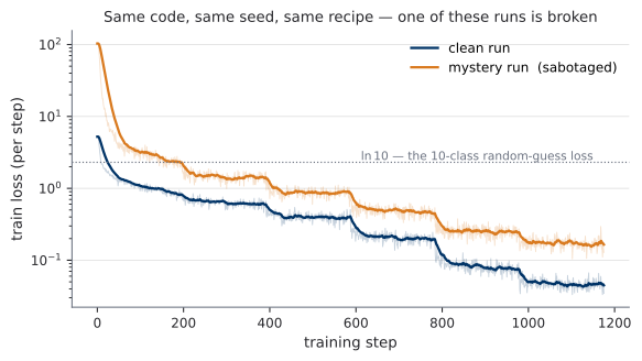
Same architecture, same optimizer, same schedule, same number of steps.

Backup slide against catastrophic laptop failure — normally students see these curves in their own MLflow UI. The annotated diagnosis lives in the notes’ post-lab debrief, NOT in this deck: do not name the bug from this slide before the reveal. Signature to point at during the reveal, live in the UI (prep numbers, seed 0): initial loss ≈97 vs ≈4.9 — a factor of 20, 40× above the ln(10) random-guess line; “ignorant, not confidently wrong” is the tell that scale is off. Grad norms elevated ~20× everywhere UPSTREAM of the bug (first conv ×21) while the head’s own gradient barely moves; head weight norm ×20 in the per-epoch logs; final acc 69.8% vs 84.5% at equal steps. Debrief bonus in the notes: the unnormalized-inputs bug was planted first and produced NO signature (BN absorbs it) — tell that story at the reveal, it lands.

The lesson

You debugged a model without reading its config. In U2 and U3 the models get stranger, but the curves speak the same language. Log first, hypothesize second, discriminate cheaply third.

This is why Block B’s checklist exists: at minute 50 you diagnosed only what someone had logged at minute 20.

• In U2/U3 you cannot eyeball a velocity field and see the bug.
• You can read its loss, its grad norms, its NFE, its throughput.
• The instrument panel is the same; only the aircraft changes.

Deliver the boxed line verbatim — it is the session’s contract with the rest of the course. Fast finishers during Block E get a second sabotaged run (same five-step task, different pathology — to be planted at prep time; see the L2-U0 sync note).

06Baseline and freeze

Launch the clean baseline

Everything, together, once:

python train_cifar.py --config configs/baseline.yaml

• Short run, live (5–8 epochs — curves, not accuracy, are the object).
• In the compare view: overlay your live run against the 30-epoch reference that shipped inside mystery-runs.zip.
• Your curve should trace the reference’s early epochs. If it does not, you now own the diagnostic toolkit to say why.

CPU-fallback configs tested in advance; throughput logging makes the fallback visible in the UI — call that out if it happens to anyone.

Freeze: the hygiene stack

hygiene-stack = training-loop-template v2 (config-driven + MLflow + schedules + checkpoint discipline) + the what-to-log checklist + the reproducibility checklist.

• Commit it now. This exact code trains every model you build in this course.
• PS0 requires, verbatim: “trained with the hygiene stack.” Config + seed + commit + MLflow store in the submission make that claim checkable.
• Deviations from the stack in later labs: permitted in writing, with a reason — same rule as the recipe card.

What’s next

• Next session (U0.T3): we go latent. Latent-variable models, the ELBO, and the VAE — the first models of the course that generate.
• The hygiene stack is assumed from here on — never re-taught, always required.
• Your CIFAR-10 baseline keeps training tonight; look at its curves tomorrow. You know how now.

End 2 minutes early if possible: the commit in Block F is the deliverable — walk the room and check git log over shoulders.