U0.L3 — VAE on MNIST
Session U0.L3 · date: see calendar-map
Today you train the first generative model of this course. The previous theory session (U0.T3) put every piece on the table — the latent-variable frame, the ELBO and its gap identity, the reparameterization trick — and assembled them into an object on paper. This session turns that object into approximately eighty lines of code, trains it on MNIST with the hygiene-stack from U0.L2, and then looks at what it learned.
The looking is the point. A VAE with a two-dimensional latent space is one of the few generative models whose entire internal representation fits on a single sheet of paper, and the picture you will produce — a plane of latent codes on which the digits arrange themselves into regions, and a decoder that turns any point of that plane into an image — is the picture this whole course is about. U1 will make that map invertible; U2 will make it a flow in continuous time; U3 will learn its velocity. Today it is a plane and a decoder, and you can see all of it.
The session produces vae-mnist-scratch, and the interfaces are frozen at the end because PS0 extends this exact codebase: your U0.L4 U-Net replaces the encoder, your U0.L4 harness evaluates the result. Design for that swap from the first cell.
Format shift, back the other way. U0.L2 was scripts and a terminal, because the object of study was the run. Today is a notebook (lab-u0l3.ipynb) again, because the object of study is code you are still shaping — and because half the session is spent looking at pictures that a notebook shows inline. Training itself still calls the hygiene-stack Trainer and still logs to MLflow: the notebook imports common/, and never copy-pastes it.
Standing reference for the modelling choices below: Bishop and Bishop (Bishop and Bishop 2024). The architecture is ours; the objective is (Kingma and Welling 2014).
Every number in these notes was measured. The runs behind the figures live in scripts/python/fig_u0_l3_vae.py, seeded, and the values they produced are recorded in scripts/python/_outputs/u0l3_vae.json. Two of this session’s claims came out differently from what the plan expected, and both are reported here as they came out — the posterior-collapse discussion in Section 6 is the more interesting one.
A · Skeleton and decisions
Reused in: PS0, directly — this is the codebase the problem set extends.
The decision nobody writes down
Before any architecture, one modelling choice has to be made explicitly, because getting it wrong is silent: what likelihood does the decoder define? U0.T3 wrote \(p_\theta(x \mid z)\) and never committed to a family. Two are standard for images.
Bernoulli decoder on binarized data. Pixels are binary, \(x_i \in \{0,1\}\), and the decoder outputs one probability per pixel: \[ \begin{aligned} p_\theta(x \mid z) &= \prod_{i=1}^{784} \mathrm{Bern}\big(x_i;\, \pi_\theta(z)_i\big), \\[2pt] -\log p_\theta(x \mid z) &= \sum_{i=1}^{784} \mathrm{BCE}\big(x_i, \pi_\theta(z)_i\big). \end{aligned} \]
Gaussian decoder, \(p_\theta(x \mid z) = \mathcal{N}(x; g_\theta(z), \sigma^2 I)\), gives a squared error and needs a variance \(\sigma^2\) that is either fixed by hand (and then silently reweights the ELBO) or learned (and then likes to run away toward zero).
We choose Bernoulli, and therefore we must supply binary data — which MNIST is not.
MNIST pixels are grayscale in \([0,1]\). Feeding them to a Bernoulli likelihood is the classic silent pairing bug: binary cross-entropy accepts fractional targets without complaint, computes something perfectly well-defined, and that something is no longer the log-likelihood of any model. The fix is dynamic binarization — every time an image is drawn, resample it:
def binarize(x):                      # x: (B, 1, 28, 28) grayscale in [0, 1]
    return torch.bernoulli(x)         # a fresh binary draw EVERY epoch
Resampling per draw rather than binarizing once is a small extra: it makes the training distribution the true Bernoulli mixture rather than one arbitrary thresholded copy of it, and it acts as free data augmentation. It is the standard protocol for likelihood numbers on MNIST, which matters because we are about to report likelihood-like numbers and want them comparable to anyone else’s.
Architecture, deliberately plain
A small convolutional encoder, a mirrored transposed-convolution decoder, and nothing clever:
encoder:  Conv 1->32  s2  ->  Conv 32->64  s2  ->  Conv 64->128 s2  ->  flatten
          -> two linear heads:  mu (d_z)   and   logvar (d_z)
decoder:  linear d_z -> 128x4x4  ->  ConvT ->  ConvT ->  ConvT  ->  784 logits
Three details are the U0.T2 recipe card being obeyed rather than re-decided. Normalization is GroupNorm, not BatchNorm — the card’s clause restricting BatchNorm to bootcamp classifiers applies from here on, and this is a generative model. The optimizer is AdamW at \(3 \times 10^{-4}\) with warmup–cosine, stepped per step. And the last layers are zero-initialized: both encoder heads, and the decoder’s output convolution.
That last one buys something concrete, which Section 2 cashes in.
run_name: U0L3-dz2-s0
seed: 0
model: {d_z: 2, enc_width: 32, dec_width: 64, norm: group}
opt:   {name: adamw, lr: 3.0e-4, weight_decay: 0.01}
sched: {name: warmup_cosine, warmup_frac: 0.03}
data:  {dataset: mnist, binarize: dynamic, batch_size: 256}
epochs: 15
d_z is a config field because you will train the model twice: \(d_z = 2\) for the latent-space pictures, and \(d_z = 16\) for the sample-quality contrast. Everything else is held fixed between them, so the comparison is a config diff of exactly one line — the U0.L2 discipline, immediately earning its keep.
A note on the data split. MNIST ships 60 000 training and 10 000 test images; we carve 6 000 validation images out of the training split and leave the test split alone. Every number in these notes is a validation number. The test split is read once, later, by the evaluation harness you build in U0.L4 — that is the split discipline of this course, and it is easier to keep than to repair.
B · Encoder, decoder, reparameterization
Why the encoder returns a logarithm
TODO B.1 (encoder part). Implement encode(x) -> (mu, logvar), both of shape (B, d_z).
The head returns \(\log \sigma_\varphi^2\), never \(\sigma_\varphi\). The reason is that a network head is an unconstrained linear map: it can output any real number, and \(\sigma\) must be positive. Parameterizing the logarithm makes every output legal, and pushes positivity into a single exp where it cannot be violated. The alternatives are worse in familiar ways — a softplus or a relu head can hand you \(\sigma = 0\) and a division by zero; clamping introduces a region with exactly zero gradient. The pattern is general and worth naming: parameterize the unconstrained quantity, and transform. You will meet it again wherever a network must output a variance, a rate, or a mixing weight.
The trick, as one line
TODO B.2 (reparameterization part). Implement the U0.T3 device.
\[ z = \mu_\varphi(x) + \exp\!\big(\tfrac{1}{2}\log\sigma_\varphi^2(x)\big) \odot \varepsilon, \qquad \varepsilon \sim \mathcal{N}(0, I_{d_z}). \]
def reparameterize(mu, logvar):       # both (B, d_z)
    return mu + torch.exp(0.5 * logvar) * torch.randn_like(mu)
That is the whole of the reparameterization trick, and the entire derivation of the previous theory session (U0.T3) has collapsed into one line with a randn_like in it. Shapes stay (B, d_z) from end to end; the broadcasting discipline of U0.L1 applies, and randn_like rather than randn(...) is how you avoid ever getting the shape or the device wrong.
TODO B.3 (decoder part). Implement decode(z) -> logits, shape (B, 1, 28, 28).
Return logits, not probabilities. Pair them with the with-logits form of binary cross-entropy, which computes \(\log(1 + e^{-x})\) through a stable branch instead of composing a sigmoid with a log and losing the tails to floating point. This is the same rule as log_softmax over log(softmax(...)) from U0.T1, in its second costume.
Checkpoint: is the latent standard normal at initialization?
mu, logvar = model.encode(binarize(x_fixed))
assert mu.abs().max() < 1e-6 and logvar.abs().max() < 1e-6
z = model.reparameterize(mu, logvar)
print(z.mean().item(), z.std().item())      # measured: 0.21, 1.09
This is the zero-initialization clause of the recipe card, paying out. With both heads zero-initialized, at step zero \(\mu_\varphi \equiv 0\) and \(\log\sigma^2_\varphi \equiv 0\), so \(\sigma_\varphi \equiv 1\) and \(z = \varepsilon\) exactly: the encoder starts life as the prior. The KL term starts at exactly zero and has to be earned, which is what makes the training curves in Section 4 readable as a story rather than a scramble.
The printed mean of \(0.21\) is not a violation — it is \(128\) draws from \(\mathcal{N}(0,1)\), whose sample mean carries a standard error of \(0.09\). The assert is on \(\mu\) and \(\log\sigma^2\), which are exact; the printout is a sanity check, and knowing which of the two to trust is itself the lesson.
C · The ELBO in code
Reused in: PS0 verbatim.
The objective is U0.T3’s, negated so it is a loss:
\[ \begin{aligned} \mathcal{L}(\theta, \varphi; x) &= \underbrace{-\,\mathbb{E}_{\varepsilon \sim \mathcal{N}(0,I)} \big[\log p_\theta(x \mid z_\varphi(x,\varepsilon))\big]}_{\text{reconstruction}} \\[4pt] &\quad + \underbrace{\mathrm{KL}\big(q_\varphi(z \mid x)\,\big\|\,p(z)\big)}_{\text{regularization}} . \end{aligned} \tag{1}\]
Both terms are computable, and the session’s hardest bug lives in how you add them up.
The reduction convention, which is the whole lesson
TODO C.1 (reconstruction part). Reconstruction is a sum over the 784 pixels, then a mean over the batch.
Equation 1 is a per-example quantity: a log-likelihood of a whole image, and a KL between two distributions on the whole latent. Both are sums over their dimensions. The batch is a Monte Carlo estimate of \(\mathbb{E}_{x \sim q}\), so the batch — and only the batch — gets a mean.
per_pixel = F.binary_cross_entropy_with_logits(logits, x, reduction="none")
recon = per_pixel.flatten(1).sum(dim=1).mean()      # sum pixels, mean batch
kl    = kl_per_dim.sum(dim=1).mean()                # sum dims,   mean batch
Reduce the reconstruction by mean over pixels instead — which is PyTorch’s default — and you have divided that term by \(784\) while leaving the KL alone. That is not a scaling of the loss. It is a different objective: a \(\beta\)-VAE with \(\beta = 784\), which nobody asked for and which the loss curve will not tell you about, because a smaller number still looks like progress.
This is not a hypothetical. Training the identical model with the identical seed and only the reduction changed:
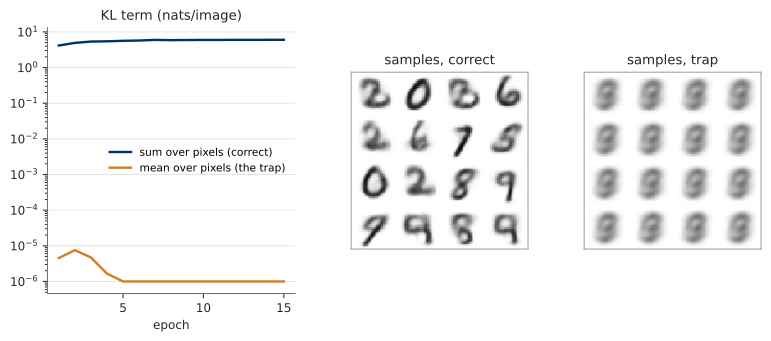
mean over pixels it falls to numerical zero within five epochs and never returns. Right: prior samples from both models, decoded from the same latent draws. The trap model has learned to ignore \(z\) entirely, so all sixteen samples are the same image — the dataset mean, which is the best a decoder can do when its input carries no information.
The measured KL of the trap run is exactly \(0.000\) nats against the correct run’s \(6.017\). The encoder has been driven to return the prior for every input; the latent is dead; the decoder outputs one image. And note what did not happen: nothing crashed, no loss went to NaN, and the reported loss decreased smoothly from \(0.274\) to \(0.264\) over fifteen epochs. The run looks healthy. That is precisely why this convention is worth a warning box instead of a footnote — and it is the same lesson as the U0.L2 mystery run, one level up: you have to know what a correct curve looks like before a wrong one can look wrong.
The KL term, per dimension
TODO C.2 (KL part). Implement the closed form, and keep it per-dimension.
For a diagonal Gaussian against \(\mathcal{N}(0, I_{d_z})\), U0.T3 quoted (and UP.A derives):
\[ \mathrm{KL}\big(q_\varphi(z\mid x)\,\big\|\,p(z)\big) = \frac{1}{2}\sum_{j=1}^{d_z} \Big(\mu_j^2 + \sigma_j^2 - 1 - \log \sigma_j^2\Big). \tag{2}\]
def kl_diag_gaussian(mu, logvar):     # -> (B, d_z), NOT summed
    return 0.5 * (mu.pow(2) + logvar.exp() - 1.0 - logvar)
Return the (B, d_z) tensor and sum it at the call site. Summing inside the function would be tidier and would throw away exactly the information Section 6 needs: which individual dimensions are doing work. Instrumentation you did not keep is instrumentation you do not have.
TODO C.3 (assembly part). Assemble the loss so that it returns its parts:
return {"loss": recon + kl, "recon": recon, "kl": kl, "kl_per_dim": kl_per_dim}Any loss that is a sum of terms returns and logs those terms separately, never only the total. A single scalar cannot distinguish “reconstruction improved” from “the KL collapsed”, and those are opposite events with the same effect on the total. The rule was stated in U0.T2’s recipe card; from here it is enforced by the interface — the loss returns a dictionary, and the Trainer logs every key.
It is not bookkeeping for its own sake: in U3 you will train a flow-matching model whose loss is an expectation over a time, a noise sample, and a data sample, and the per-part decomposition is the only cheap instrument you will have.
The gradient-check ritual, on a stochastic loss
Reused in: U3.L1, on the CFM loss — this is the first of several.
U0.L1 established the ritual: after writing a loss by hand, verify its gradient against finite differences in float64 before trusting a single training step. The ELBO adds a wrinkle, because it is a random function — evaluating it twice gives two different numbers, and differencing two independent draws measures noise.
eps = torch.randn(B, d_z, dtype=torch.float64)   # drawn ONCE, reused

def loss_at(w):                       # deterministic given eps
    param.copy_(w);  mu, logvar = model.encode(x)
    z = mu + torch.exp(0.5 * logvar) * eps       # <- the fixed draw
    return recon(model.decode(z), x) + kl(mu, logvar)

numeric  = (loss_at(w + h) - loss_at(w - h)) / (2 * h)
analytic = autograd_grad_of(loss_at, w)
Freezing \(\varepsilon\) turns the estimator into an ordinary deterministic function of the parameters, and the reparameterization is exactly what makes that legal: the randomness is now an input, and inputs can be held fixed. The check ran at a maximum relative error of \(1.6 \times 10^{-7}\).
Two traps are worth your attention, because the first one caught the preparation of this very session.
A check run at initialization cannot fail. The heads are zero-initialized, so at step zero the gradient reaching any encoder body parameter is exactly zero. Analytic zero, numeric zero, relative error reported as \(0.0\) — a perfect score from a measurement of nothing. Take a few optimizer steps first, and assert that the analytic gradient is nonzero before believing that it agrees with anything.
A check that has never failed is not known to work. So make it fail on purpose. Dropping the \(\tfrac{1}{2}\) from Equation 2 — a plausible typo — and re-running the ritual against the correct finite differences gives a maximum relative error of \(1.0\): total disagreement, instantly. That is what a working check looks like when it fires, and now you have seen it do so.
D · Training with the hygiene stack
Nothing here is new machinery; that is the payoff of U0.L2. The config is read, the Trainer is constructed, the run is tagged session: U0.L3, and the three loss parts are logged per step.
mlflow.set_tracking_uri("sqlite:///mlflow.db")
mlflow.set_experiment("fbgm-2026")
with mlflow.start_run(run_name=cfg.run_name):
    mlflow.log_params(flatten(cfg))
    mlflow.set_tags({"session": "U0.L3", "tag": f"dz{cfg.d_z}", "seed": cfg.seed})
    trainer.fit(train_loader, val_loader, epochs=cfg.epochs)
TODO D.1 (logging part). Add two per-epoch mlflow.log_figure calls: a reconstruction grid on a fixed validation batch, and a prior-sample grid from a fixed bank of \(\varepsilon\) draws.
Both words fixed are load-bearing. Panels are only comparable across epochs — and across runs, and across your classmates’ runs — if the inputs that produced them are identical; a fresh noise draw each epoch produces a slideshow in which you cannot tell improvement from reshuffling. Commit the batch and the noise bank as tensors. The same trick reappears for sample panels in the U3 labs, where the models are slow enough that a wasted comparison costs real time.
Reading the curves while it trains
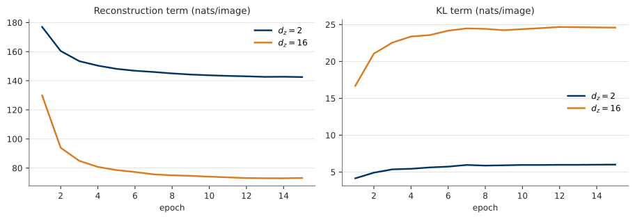
The \(d_z = 2\) run ends at \(142.6\) nats of reconstruction and \(6.0\) nats of KL; the \(d_z = 16\) run at \(73.1\) and \(24.6\). Read that as an information budget: the wider latent is allowed to carry roughly four times as much information about \(x\), and it spends it buying about half the reconstruction cost.
The shape of the KL curve is the part worth pausing on. It rises — monotonically, from zero — even though the objective is minimizing a sum containing it. Nothing is broken. The KL is the price the model pays for a latent that is informative, and the reconstruction term is willing to pay it. If your KL curve instead falls to zero, you are looking at Figure 1.
E · The latent space
This is the session’s payoff, and it needs the \(d_z = 2\) model, because two dimensions can be drawn.
Clusters that no label produced
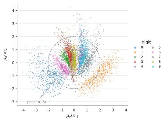
Three things to read off Figure 3, in order of how much they matter later.
The digits separate without supervision. Nothing in Equation 1 mentions a class; the only pressure is that the decoder must rebuild the image from \(z\), and images that look alike must therefore land near each other. This is representation learning arriving as a side effect, and it is the reason latent-variable models were interesting long before they generated anything convincing.
The cloud sits roughly where the prior does. That is the KL term at work: it is pulling the aggregate of all the \(q_\varphi(z\mid x)\) toward \(\mathcal{N}(0,I)\), and it has to succeed, because generation samples from the prior. A latent cloud that drifted away from the prior would mean that the codes the decoder was trained on and the codes it will be asked to decode are different populations.
And the separation is imperfect — the \(4\)/\(9\) and \(3\)/\(5\) neighbourhoods overlap, and some points sit far out. With two dimensions there is nowhere else for them to go. That is a statement about the capacity of \(d_z = 2\), not about the method.
The decoder as a map of the plane
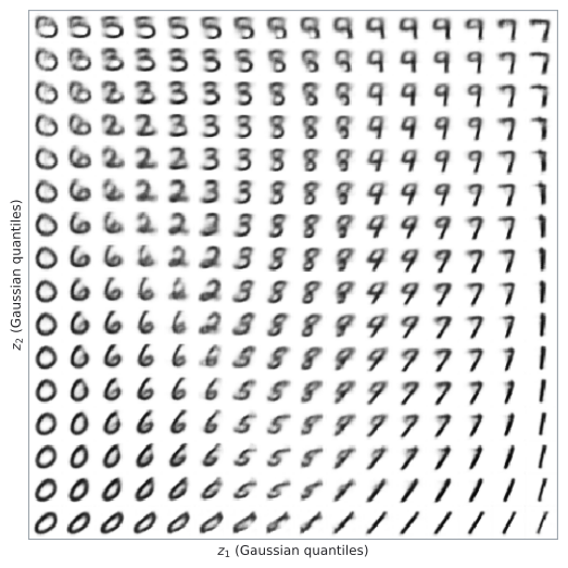
Figure 4 is the picture to carry out of this session. The decoder has turned a featureless Gaussian plane into an organized atlas of handwritten digits, and it is continuous: walk in any direction and the digit deforms smoothly into its neighbours, passing through shapes that are not quite any digit on the way.
The animation below runs both panels together over the real checkpoints of this same run — encoder side and decoder side advancing in step, so the scatter and the sheet are visibly two views of one object. It also settles a question the static figures cannot: in what order do the ELBO’s two terms do their work.
Two phases, and the readouts on screen are what distinguish them. First the KL inflates the cloud from a single point out to the prior’s scale — the mean radius \(\mathrm{RMS}\lVert\mu_\varphi\rVert\) climbs from \(0\) to about \(1.2\) within the first epoch. Then it stops: across epochs 1 to 15 that radius stays between \(1.20\) and \(1.31\), pinned, while the cluster-separation statistic goes on climbing from \(1.58\) to \(2.21\). The KL sets the scale and then holds it; reconstruction does its organizing inside a budget that no longer moves.
The first sixty steps carry a magnification badge, because they happen at roughly a thousandth of the panel’s scale — the shape is already half-organized while the cloud is still a speck, and a panel that quietly rescaled itself would be hiding exactly that.
Generative modelling, in one sentence: learn a map from a simple noise distribution to the data distribution. Figure 4 is that map, drawn in full for \(d_z = 2\).
Everything ahead is a different answer to how to build the map. U1 makes it invertible, so the change-of-variables formula gives exact likelihoods. U2 makes it a flow in continuous time — the map becomes the solution of an ODE rather than a stack of layers. U3 learns the velocity of that flow directly and stops simulating it during training.
The VAE’s map is none of those things: it is a single feed-forward decoder, trained through a bound, and it is blurry. Keep the picture; we are about to spend a semester improving the mechanism behind it.
Walking between two digits
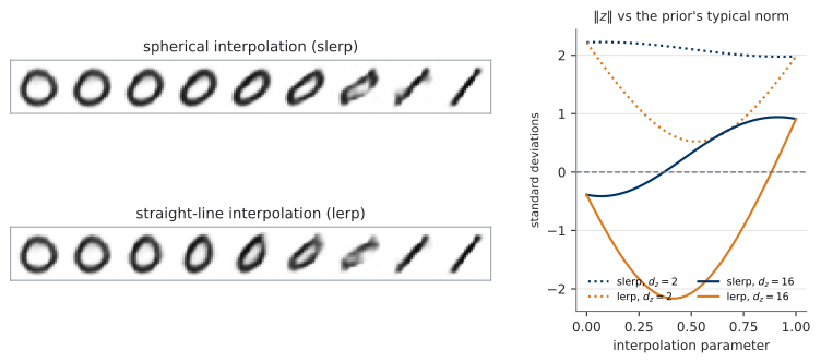
TODO E.1 (interpolation part). Encode two validation images, interpolate between their \(\mu_\varphi\), decode the path.
The standard advice is to use spherical interpolation for Gaussian latents, and the standard justification is that the straight line between two codes dips toward the origin, through a low-norm region the decoder rarely saw. Half of that is right, and it is worth getting the other half correct because the reasoning recurs.
For \(z \sim \mathcal{N}(0, I_d)\), the norm \(\|z\|\) concentrates: its mean grows like \(\sqrt{d}\) while its standard deviation stays near \(1/\sqrt{2}\) regardless of \(d\). So “off the typical set” has to be measured in units of that spread, not in raw norm. Measured on our own runs, at the midpoint of the path:
| \(d_z = 2\) | \(d_z = 16\) | |
|---|---|---|
| straight line (lerp) | \(0.53\sigma\) below typical | \(2.07\sigma\) below typical |
| spherical (slerp) | \(2.10\sigma\) above typical | \(0.32\sigma\) above typical |
At \(d_z = 16\) the folklore holds exactly: lerp’s midpoint is two standard deviations too short, slerp’s sits essentially on the typical shell. At \(d_z = 2\) it inverts — our two endpoints happen to lie far out in the plane, slerp faithfully holds the entire path at that atypical radius, and it is the spherical path that is two standard deviations off. The dip’s size is set by the angle between the endpoints; what grows with dimension is how many standard deviations that dip is worth.
The \(d_z = 2\) row is worth distrusting on principle, and the lab will show you why: with two dimensions the deviation depends on which pair of images you happened to pick and on the particular run, and it changes sign between the run behind this table and the one the lab notebook produces. That instability is itself the point. Slerp’s justification is a concentration argument, concentration is a high-dimensional phenomenon, and \(d_z = 2\) is the wrong place to go looking for it. The \(d_z = 16\) column is the one to trust.
So: use slerp in the latent spaces you will meet later, which are high-dimensional, and know the reason rather than the rule. And notice that the decoded rows in Figure 5 look the same either way — at \(d_z = 2\) this choice does not matter, and a figure that pretended otherwise would be a nicer figure and a false one.
What a wider latent buys
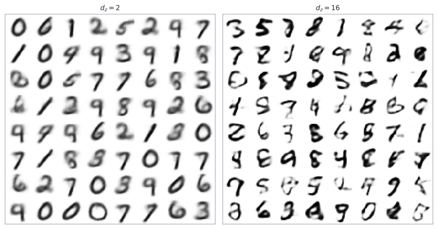
The \(d_z = 16\) samples are visibly better: more of them are digits, and the strokes are sharper. Its latent space, however, cannot be drawn, and no amount of cleverness recovers Figure 3 from sixteen dimensions — a projection of it is a projection, not the map. That is the trade in one sentence: interpretability is a property of small latent spaces, and sample quality is not. No setting reconciles them; you pick a dimension for the job you have.
Both sets of samples are also blurry, which is not a bug you can tune away. The model is optimizing a bound, its decoder is a factorized Bernoulli that cannot express correlations between pixels given \(z\), and averaging over the posterior smooths what remains. U0.T4 gives you the vocabulary to say how much worse this is than a sharper model, and U0.L4 gives you the number.
F · Posterior collapse, in passing
Five minutes, and the L3 plan asked for a specific phenomenon: with \(d_z = 16\), several latent dimensions’ KL should sit at essentially zero, ignored by the decoder. Pull up the per-dimension KL you carefully kept in TODO C.2 and look.
It does not happen. Not one of the sixteen dimensions is unused; the quietest carries \(1.06\) nats, a hundred times above the conventional \(0.01\)-nat threshold for calling a dimension dead. On this model, on this data, at this width, \(d_z = 16\) is not enough latent space to waste any.
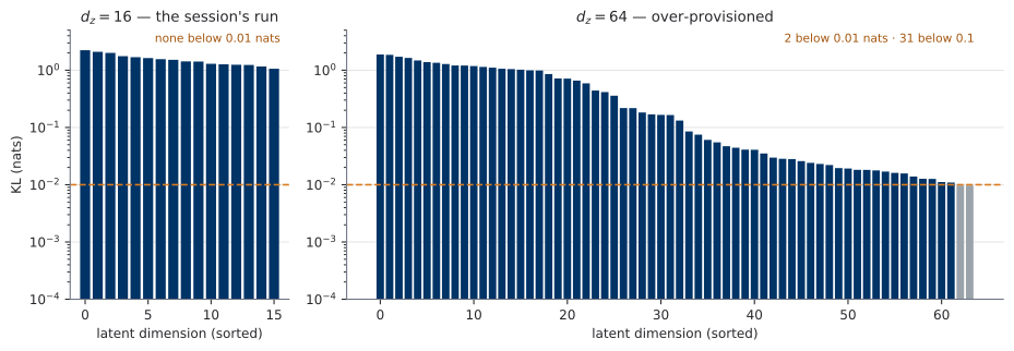
So the phenomenon is real, and finding it required asking what actually causes it. Sweeping the latent dimension with everything else held fixed:
| \(d_z\) | dead (\(<0.01\) nats) | nearly dead (\(<0.1\)) | total KL | reconstruction |
|---|---|---|---|---|
| 16 | 0 | 0 | 24.6 | 73.1 |
| 32 | 0 | 0 | 30.1 | 68.5 |
| 64 | 2 | 31 | 30.5 | 69.3 |
| 128 | 34 | 99 | 30.3 | 70.0 |
| 64, decoder \(2.5\times\) wider | 10 | 32 | 30.2 | 66.9 |
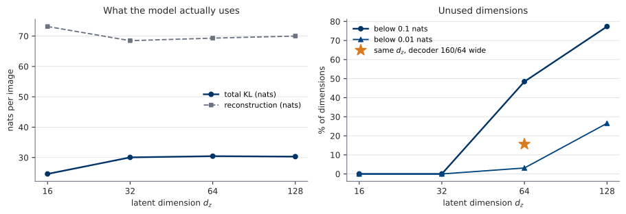
Table 1 says something sharper than “collapse happens”. The total KL saturates at about \(30\) nats and stays there — \(30.1\), \(30.5\), \(30.3\) as the latent goes \(32 \to 64 \to 128\) — and the reconstruction is flat alongside it. The model has an information budget set by what its decoder can use, and beyond that point extra dimensions are not used badly; they are not used at all. Posterior collapse is what surplus capacity looks like from the inside.
The mechanism. If the decoder can reconstruct just as well while ignoring coordinate \(j\) of \(z\), then coordinate \(j\) contributes nothing to the reconstruction term — and the KL term is a cost, minimized at \(q_\varphi(z_j \mid x) = p(z_j)\). So the encoder switches that coordinate off. It is not pathological optimization; it is the objective being minimized correctly.
The second lever, isolated. Holding \(d_z = 64\) and widening only the decoder (\(2.5\times\)) takes dead dimensions from \(2\) to \(10\). A stronger decoder needs less help from \(z\), so it can afford to ignore more of it — the mechanism, controlled.
Mitigations, named and not implemented: KL annealing (ramp the KL weight from zero), and free bits (exempt a small per-dimension KL budget from the penalty). Both are \(\beta\)-VAE-family reweightings, both are one line, and both are out of scope today.
Scope. Everything above is \(15\) epochs of one architecture on MNIST at one seed. The direction of the effect is robust and mechanical; the exact thresholds are not portable, and reporting them as if they were would be the kind of claim this course keeps asking you to interrogate.
The moral, and the reason this is the last block rather than a footnote: you could only see any of this because you logged the KL per dimension. The aggregate KL of the \(d_z = 64\) run is \(30.5\) nats — a perfectly healthy-looking number, indistinguishable from the \(d_z = 32\) run’s \(30.1\), and it conceals the fact that half the model is inert. The instrument was one line in TODO C.2, kept rather than summed away.
Freeze the artifact
Interface contract, binding for PS0:
encode(x)                  -> (mu, logvar)     # both (B, d_z)
reparameterize(mu, logvar) -> z                # (B, d_z)
decode(z)                  -> logits           # (B, 1, 28, 28)
loss(x)   -> {"loss", "recon", "kl", "kl_per_dim"}
Reconstruction is summed over pixels; KL is summed over dimensions; both are averaged over the batch. Data is dynamically binarized. Commit and tag u0l3-freeze.
The contract is written this way for one reason: PS0 replaces encode and nothing else. Your U0.L4 U-Net encoder will return the same (mu, logvar) pair with the same shapes, drop into the same loss, and train under the same Trainer — no surgery. Interfaces designed one session ahead of the swap are the difference between an assignment and an afternoon of rewriting.
Take vae-mnist-scratch and:
- replace the encoder with your
unet-skeleton(U0.L4), - train it with the
hygiene-stack(U0.L2) — config, seed, commit, MLflow store, - evaluate it with your
eval-harness(U0.L4) — FID at the course-standard sample count, plus sample panels.
Graded on correctness and reproducibility, not on how good the samples look. A model that scores poorly and is fully reconstructible from its logged run scores better than a pretty one that is not.
Where this goes next
The next theory session (U0.T4) is architectures for the road: attention in one pass, the U-Net, and — the part that matters most for everything after U0 — time and positional embeddings. Every model from U2 onward is conditioned on a time \(t\), and how you feed a scalar time into a convolutional network is a specific technique with a specific name, not an implementation detail. That session also defines FID, which is how U0.L4 will finally put a number on the samples in Figure 6.
Two threads from today run all the way to the end of the course. The first is Figure 4: a map from noise to data, which is what every model in this course is, and which the next three units rebuild with progressively better machinery. The second is smaller and just as durable — a composite loss logs its parts, and an instrument you summed away is an instrument you do not have. It cost one line today. In U3 it will be the only thing standing between you and a silently wrong velocity field.
Further reading
- (Bishop and Bishop 2024), the chapters on latent-variable models and deep generative models — closest to this session’s level and notation.
- (Kingma and Welling 2014) — the original, and still the clearest statement of the amortized-inference argument; §2.4 is the objective implemented above.
- (Murphy 2023) — more depth on variational inference, including the \(\beta\)-VAE family whose mitigations were named in Section 6 and not implemented.