U0.L3 — VAE on MNIST

Flow-Based Generative Models · UFRJ · 2026.2

01Skeleton and decisions

Today you train the first generative model

The previous theory session (U0.T3) assembled the VAE on paper: latent variables, the ELBO and its gap, reparameterization.

Today it becomes ~80 lines of code, trained with the hygiene stack.

Then we look at it — and a \(d_z = 2\) VAE is one of the few generative models whose entire internal representation fits on one sheet of paper.

Produces vae-mnist-scratch — frozen at the end, because PS0 extends this exact code: your U0.L4 U-Net replaces the encoder.

One minute. The framing that matters: today is the first time they see the picture the whole course is about (noise plane -> data), and everything after U0 is a better mechanism for building that same map. Say the PS0 sentence early — it changes how carefully they write the interfaces.

Why a notebook again

U0.L2 was scripts, because the object of study was the run.

Today is lab-u0l3.ipynb, because the object of study is code you are still shaping — and half the session is pictures.

Training still calls the hygiene-stack Trainer and still logs to MLflow. The notebook imports common/; it never copies it.

model: {d_z: 2, enc_width: 32, dec_width: 64}
opt:   {name: adamw, lr: 3.0e-4, weight_decay: 0.01}
data:  {dataset: mnist, binarize: dynamic, batch: 256}

d_z: 2 for the pictures · d_z: 16 for sample quality.

The decision nobody writes down

U0.T3 wrote \(p_\theta(x \mid z)\) and never chose a family. You must.

Bernoulli on binary pixels: decoder outputs one probability per pixel; \(-\log p_\theta(x\mid z)\) is a binary cross-entropy.

Gaussian: squared error, plus a \(\sigma^2\) you fix by hand (and silently reweight the ELBO) or learn (and watch run to zero).

We choose Bernoulli — so the data must be binary, and MNIST is not.

def binarize(x):        # x in [0,1], (B,1,28,28)
    return torch.bernoulli(x)   # fresh draw EVERY epoch

Name the silent bug explicitly: BCE accepts fractional targets without complaint and computes something well-defined that is not the log-likelihood of any model. Nothing errors. Dynamic (per-draw) binarization rather than thresholding once: it is the standard protocol, and it is free augmentation.

Architecture, deliberately plain

enc: Conv 1->32 s2 -> 32->64 s2 -> 64->128 s2
     -> flatten -> two heads: mu (d_z), logvar (d_z)
dec: linear -> 128x4x4 -> ConvT x3 -> 784 logits

Three details are the U0.T2 recipe card, obeyed, not re-decided:

• GroupNorm, not BatchNorm — the BN clause was for bootcamp classifiers; this is a generative model,
• AdamW \(3\times10^{-4}\), warmup–cosine, stepped per step,
• zero-init last layers — both heads and the decoder output.

That last one pays out two slides from now.

Also state the split discipline: 6k validation carved out of the 60k train split, test split untouched until the U0.L4 harness reads it once. Every number today is a validation number.

02Encoder, decoder, reparameterization

TODO B.1 — why the head returns a logarithm

The encoder returns \(\log \sigma_\varphi^2\), never \(\sigma_\varphi\).

A network head is an unconstrained linear map — it can emit any real number. But \(\sigma\) must be positive.

Parameterize the logarithm: every output is legal, and positivity lives in a single exp where it cannot be violated.

• softplus/relu head \(\to\) can hand you \(\sigma = 0\), then a division,
• clamping \(\to\) a region with exactly zero gradient.

The pattern, which recurs: parameterize the unconstrained quantity and transform. (Variances, rates, mixing weights.)

TODO B.2 — the trick, as one line

\[ z = \mu_\varphi(x) + \exp\!\big(\tfrac12 \log\sigma^2_\varphi(x)\big) \odot \varepsilon, \qquad \varepsilon \sim \mathcal{N}(0, I_{d_z}) \]

def reparameterize(mu, logvar):      # both (B, d_z)
    sigma = torch.exp(0.5 * logvar)
    return mu + sigma * torch.randn_like(mu)

The whole derivation of U0.T3 has collapsed into one line with a randn_like in it.

TODO B.3 (decoder part): return logits, not probabilities — pair with the with-logits BCE. Same rule as log_softmax in U0.T1, second costume.

Shapes stay (B, d_z) end to end — U0.L1 broadcasting discipline. randn_like rather than randn(…): you can never get the shape or the device wrong.

Checkpoint — is the latent standard normal at init?

mu, logvar = model.encode(binarize(x_fixed))
assert mu.abs().max() < 1e-6
assert logvar.abs().max() < 1e-6
z = model.reparameterize(mu, logvar)
print(z.mean().item(), z.std().item())   # 0.21, 1.09

Zero-init heads \(\Rightarrow\) \(\mu_\varphi \equiv 0\), \(\sigma_\varphi \equiv 1\), so \(z = \varepsilon\) exactly: the encoder starts as the prior.

The KL term starts at exactly zero and has to be earned — which is what makes the training curves readable later.

The printed 0.21 is not a violation: 128 draws from N(0,1), standard error 0.09. The assert is on mu and logvar, which are exact; the printout is a sanity check. Knowing which of the two to trust is the lesson.

03The ELBO in code

The objective, negated into a loss

\[ \mathcal{L}(\theta,\varphi;x) = \underbrace{-\,\mathbb{E}_{\varepsilon \sim \mathcal{N}(0,I)} \big[\log p_\theta(x \mid z_\varphi(x,\varepsilon))\big]}_{\text{reconstruction}} \;+\; \underbrace{\mathrm{KL}\big(q_\varphi(z\mid x)\,\|\,p(z)\big)}_{\text{regularization}} \]

Both terms are computable. The session’s hardest bug is in how you add them up.

TODO C.1 — the reduction convention

The loss is a per-example quantity: both terms are sums over their own dimensions. Only the batch gets a mean.

recon = per_pixel.flatten(1).sum(dim=1).mean()
kl    = kl_per_dim.sum(dim=1).mean()

Reduce reconstruction by mean over pixels — PyTorch’s default — and you divided that term by \(784\) and left the KL alone.

That is not a rescaling. It is a different objective: a \(\beta\)-VAE with \(\beta = 784\), which nobody asked for.

This is the planted lesson of the lab — not a sabotage, a convention they will get wrong. Do NOT tell them the consequence yet; the next slide shows the measured run. Let someone predict what happens first.

What the wrong reduction actually does

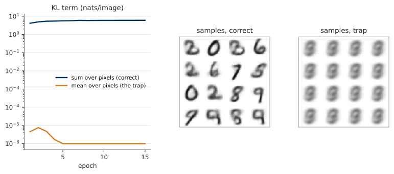
Same model, same seed, only the reduction changed. KL falls to \(0.000\) nats in five epochs; all sixteen samples are one image — and nothing crashed: the loss fell smoothly, \(0.274 \to 0.264\).

The run LOOKS HEALTHY. That is why this gets a warning box, not a footnote, and it is the U0.L2 mystery-run lesson one level up: you have to know what a correct curve looks like before a wrong one can look wrong. The decoder has learned to ignore z, so it outputs the dataset mean — the best it can do when its input carries no information.

TODO C.2 — the KL, kept per dimension

\[ \mathrm{KL}\big(q_\varphi(z\mid x)\,\|\,p(z)\big) = \frac12 \sum_{j=1}^{d_z}\big(\mu_j^2 + \sigma_j^2 - 1 - \log\sigma_j^2\big) \]

Derived in UP.A; today it is a tool.

def kl_diag_gaussian(mu, logvar):    # -> (B, d_z)
    return 0.5*(mu.pow(2) + logvar.exp() - 1.0 - logvar)

Return the (B, d_z) tensor. Sum at the call site.

Summing inside would be tidier and would throw away exactly what the last block of this session needs.

TODO C.3 — a loss that returns its parts

return {"loss": recon + kl, "recon": recon,
        "kl": kl, "kl_per_dim": kl_per_dim}

A single scalar cannot distinguish “reconstruction improved” from “the KL collapsed” — opposite events, same effect on the total.

Stated in U0.T2’s recipe card; from here it is enforced by the interface. The Trainer logs every key.

In U3 your loss is \(\mathbb{E}_{t,\,x_0,\,x_1}[\,\cdot\,]\) and this decomposition is the only cheap instrument you will have.

The gradient-check ritual, on a random loss

U0.L1’s rule: check a hand-written loss against finite differences in float64 before trusting a training step. But the ELBO is a random function — differencing two independent draws measures noise.

eps = torch.randn(B, d_z, dtype=torch.float64)  # ONCE

def loss_at(w):            # deterministic given eps
    param.copy_(w)
    mu, logvar = model.encode(x)
    z = mu + torch.exp(0.5*logvar) * eps        # the fixed draw
    return recon(model.decode(z), x) + kl(mu, logvar)

Reparameterization is why this is legal: randomness is an input.

Freezing eps turns the estimator into an ordinary deterministic function of the parameters. Without it you difference two independent draws and measure noise. Point at the fact that this is the trick from Block B paying a debt they did not know they had.

Two traps — and this one caught us

Measured: max relative error \(1.6\times10^{-7}\). Good. But:

Zero-init heads \(\Rightarrow\) the gradient reaching any encoder body parameter is exactly \(0\) at step \(0\). Analytic \(0\), numeric \(0\), error reported as \(0.0\) — a perfect score from measuring nothing.

Take a few optimizer steps first; assert the gradient is nonzero before believing it agrees with anything.

A check that has never failed is not known to work. Drop the \(\tfrac12\) from the KL — a plausible typo — and re-run: relative error \(1.0\). Total disagreement, instantly.

Now you have seen it fire.

This is a real incident from preparing this session, not a hypothetical — say so. The first version of the check reported a perfect 0.0 and was measuring nothing. It is the same species as the U0.L2 negative result: verify your instruments, empirically.

04Training with the hygiene stack

Nothing new here — that is the payoff

mlflow.set_tracking_uri("sqlite:///mlflow.db")
mlflow.set_experiment("fbgm-2026")
with mlflow.start_run(run_name=cfg.run_name):
    mlflow.log_params(flatten(cfg))
    mlflow.set_tags({"session": "U0.L3", "seed": cfg.seed,
                     "tag": f"dz{cfg.d_z}"})
    trainer.fit(train_loader, val_loader, cfg.epochs)

TODO D.1 (logging part): two per-epoch mlflow.log_figure calls — a reconstruction grid on a fixed validation batch, and a prior-sample grid from a fixed bank of \(\varepsilon\).

Both “fixed” are load-bearing: a fresh draw each epoch gives a slideshow where improvement and reshuffling look identical.

Read the curves while it trains

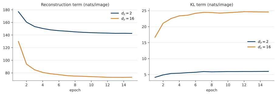
U0.T3’s tug-of-war, measured. The KL rises from zero — the encoder starts equal to the prior and buys information only as far as reconstruction pays for it.

\(d_z=2\): \(142.6 + 6.0\) nats · \(d_z=16\): \(73.1 + 24.6\) nats.

Ask why the KL rises when we are minimizing a sum containing it. Answer: the KL is the PRICE of an informative latent and reconstruction is willing to pay it. If their KL curve falls to zero instead, they are looking at the trap from Block C. Read the two runs as an information budget: 4x the KL buys about half the reconstruction cost.

05The latent space

Clusters that no label produced

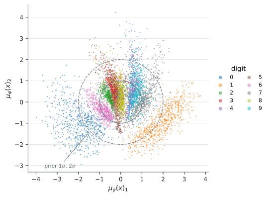
Each point is \(\mu_\varphi(x)\), colored by digit. The labels were never shown to the model — the only pressure is that the decoder must rebuild \(x\) from \(z\), so similar images land near each other.

Three readings, in order of importance later: (1) unsupervised separation — representation learning as a side effect; (2) the cloud sits where the prior does, which is the KL doing its job, and it MUST, because generation samples the prior; (3) the separation is imperfect (4/9, 3/5 overlap) — a statement about d_z = 2’s capacity, not about the method.

The decoder as a map of the plane

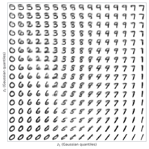
Decoder on a lattice of Gaussian quantiles — no data involved.

Watch both sides form at once

Every frame is measured — the same run as the two static figures, asserted equal to it. Two phases, and the numbers on screen are what separate them: the KL inflates the cloud from a point to the prior’s scale (RMS 0 -> 1.2), and only THEN does reconstruction reorganize inside a scale that stops moving (RMS flat 1.20-1.31 while separation climbs 1.58 -> 2.21). Point at the magnification badge: the first 60 steps happen ~1000x below the panel scale, so the panel says so rather than silently rescaling.

The picture the whole course is about

Generative modelling in one sentence: learn a map from a simple noise distribution to the data distribution.

The previous slide is that map, drawn in full for \(d_z = 2\).

Everything ahead is a different answer to how to build the map:

• U1 — make it invertible: exact likelihoods by change of variables,
• U2 — make it a flow in continuous time: the map solves an ODE,
• U3 — learn the flow’s velocity, and stop simulating during training.

The VAE’s map is a single feed-forward decoder, trained through a bound, and it is blurry. Keep the picture; we spend a semester on the mechanism.

TODO E.1 — walking between two digits

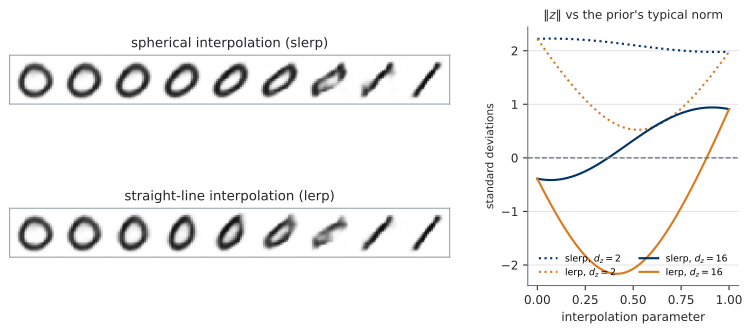
Folklore: use slerp — the straight line dips toward the origin, through a low-norm region the decoder never saw. Half right: \(\|z\|\) concentrates with spread \(\sim\!1/\sqrt2\) for every \(d\), so the deficit must be measured in those units.

The measurement, which inverts the rule

midpoint of the path	\(d_z = 2\)	\(d_z = 16\)
straight line (lerp)	\(0.53\sigma\) below	\(2.07\sigma\) below
spherical (slerp)	\(2.10\sigma\) above	\(0.32\sigma\) above

At \(d_z = 16\) the folklore holds exactly. At \(d_z = 2\) it inverts: our endpoints lie far out, slerp faithfully holds the whole path at that atypical radius.

Use slerp in high dimensions — and know the reason, not the rule.

The dip’s SIZE is set by the angle between endpoints; what grows with dimension is how many standard deviations that dip is worth. Point out that the decoded rows look identical either way at d_z = 2 — a figure that pretended otherwise would be nicer and false.

What a wider latent buys

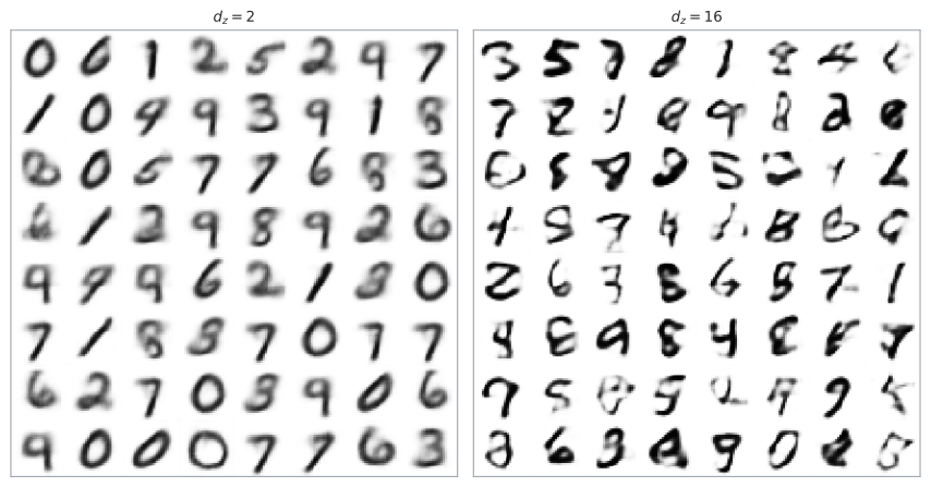
\(d_z=16\): more of them are digits, strokes sharper — and its latent space cannot be drawn.

Interpretability is a property of small latent spaces; sample quality is not. No setting reconciles them; you pick a dimension.

06Posterior collapse, and the freeze

The phenomenon we were promised

Pull up the per-dimension KL you kept in TODO C.2, \(d_z = 16\). Several dimensions should sit at \(\approx 0\), ignored by the decoder.

It does not happen. Not one of the sixteen is unused — the quietest carries \(1.06\) nats, a hundred times the \(0.01\)-nat threshold for calling a dimension dead.

At this width, on this data, \(d_z = 16\) is not enough latent space to waste any.

This is a genuine negative result from preparing the session — the pre-plan expected collapse here. Same species as U0.L2’s bug A. Do not paper over it: the phenomenon is real, and finding it means asking what actually causes it.

So ask what causes it

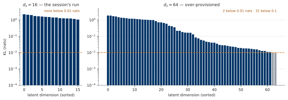
Left: the session’s \(d_z=16\) run — every dimension active. Right: \(d_z=64\) — \(31\) of \(64\) below \(0.1\) nats, \(2\) fully dead.

Capacity, swept

\(d_z\)	dead	nearly dead	total KL	recon
16	0	0	24.6	73.1
32	0	0	30.1	68.5
64	2	31	30.5	69.3
128	34	99	30.3	70.0
64, decoder \(2.5\times\) wider	10	32	30.2	66.9

Total KL saturates at \(\approx 30\) nats and stays there. The model has an information budget; beyond it, extra dimensions are not used badly — they are not used at all.

Posterior collapse is what surplus capacity looks like from inside.

Mechanism, and the honest scope

If the decoder reconstructs just as well ignoring coordinate \(j\), then \(j\) earns nothing in the reconstruction term — and the KL is a cost, minimized at \(q_\varphi(z_j\mid x) = p(z_j)\), so the encoder switches it off.

Not pathological optimization: the objective, minimized correctly.

Second lever, isolated: hold the latent at \(d_z=64\) and widen only the decoder (\(2.5\times\)) — dead dimensions go from \(2\) to \(10\). A stronger decoder needs less help from \(z\).

Named, not implemented: KL annealing, free bits. Scope: one architecture, MNIST, 15 epochs, one seed. The direction is mechanical; the thresholds are not portable.

The moral of the whole session

The aggregate KL of the \(d_z = 64\) run is \(30.5\) nats.

The \(d_z = 32\) run’s is \(30.1\).

Indistinguishable — and half of one model is inert.

You could only see this because you logged the KL per dimension. The instrument was one line in TODO C.2, kept rather than summed away.

This is the line to end the technical content on. It closes the loop opened in Block C and it is the transferable habit — in U3 it is the only thing standing between them and a silently wrong velocity field.

Freeze vae-mnist-scratch

encode(x)                  -> (mu, logvar)
reparameterize(mu, logvar) -> z
decode(z)                  -> logits
loss(x) -> {loss, recon, kl, kl_per_dim}

Recon summed over pixels; KL summed over dimensions; both averaged over the batch. Data dynamically binarized. Tag u0l3-freeze.

PS0 replaces encode and nothing else — your U0.L4 U-Net returns the same pair, with the same shapes, into the same loss.

PS0, in outline

Take vae-mnist-scratch and:

1. replace the encoder with your unet-skeleton (U0.L4),
2. train it with the hygiene-stack (U0.L2),
3. evaluate it with your eval-harness (U0.L4) — FID at the course-standard sample count, plus panels.

Graded on correctness and reproducibility, not sample quality. A weak model that is fully reconstructible from its logged run scores above a pretty one that is not.

Next session (U0.T4): architectures for the road

Attention in one pass · U-Net anatomy · time and positional embeddings — every model from U2 on is conditioned on a time \(t\), and feeding a scalar time into a convolutional network is a named technique, not an implementation detail.

It also defines FID, which is how U0.L4 finally puts a number on those blurry samples.

Two threads run from today to the end of the course: the map from noise to data — and a composite loss logs its parts.

Close on the two threads. The manifold sheet is the picture they should be able to recall in U3 when the velocity field shows up; the logging rule is the habit that survives the whole semester.