U0.T5 — Numerical ODE Solvers
Session U0.T5 · date: see calendar-map
How to read this page. These notes are written to be read alone. They are also the core of the self-study packet that PESC students receive at enrollment, so nothing here depends on having attended a live session, and nothing here depends on having attended the earlier bootcamp sessions. Every figure explains itself in its caption. Every exercise at the end carries its own answer. Every piece of code runs on a laptop CPU in seconds.
This is the last drawer of the bootcamp toolbox, and it is the one the second half of the course lives in. From U2 onward, generating a sample means solving an ordinary differential equation. The model is the right-hand side of that equation; the solver is everything else. This page is about everything else.
Standing reference for the unit: (Bishop and Bishop 2024). For the curious, and not required: the ODE-solver chapter of (Kidger 2022), which covers the same ground with the neural-network application in view from the start.
Why solvers, and why now
A generative model in this course is a velocity field. It is a function that takes a point \(x \in \mathbb{R}^d\) and a time \(t \in [0,1]\), and returns the direction and speed in which that point should move:
\[ \frac{\mathrm{d}x}{\mathrm{d}t} \;=\; u_t(x) , \qquad x(0) = x_0 . \tag{1}\]
The time convention of this course is fixed and never varies: \(t = 0\) is noise, \(t = 1\) is data. So you draw \(x_0\) from a standard Gaussian, you follow Equation 1 from \(t=0\) to \(t=1\), and whatever the trajectory reaches at \(t=1\) is your generated sample. That is the whole sampling procedure. When the field is a neural network with parameters \(\theta\), the course writes it \(u_t^\theta(x)\).
The consequence is immediate and it is the reason this session exists. You cannot follow Equation 1 exactly. You can only approximate the trajectory, by evaluating the field at finitely many points and stepping between them. Each of those evaluations is one forward pass of a neural network. So the cost of generating one sample is
\[ \text{cost} \;=\; \text{NFE} \times (\text{cost of one forward pass}) . \]
The number of function evaluations, written NFE, is the count of calls to the right-hand side \(f\) that a solver makes while it integrates from \(t_0\) to \(t_1\). It is not a diagnostic and it is not an implementation detail. In this course it is a first-class output of every solver, returned alongside the trajectory, and reported in every experiment.
NFE is the cost currency of the entire field. Whole research papers exist whose complete contribution is reducing it — same samples, fewer network calls. By the end of this course you will read several of them, and the reason their titles make sense to you will be this page.
Two words of context for a reader who has not seen the earlier bootcamp sessions. First, “a neural network” here means any parameterized function \(\mathbb{R}^d \times [0,1] \to \mathbb{R}^d\) that you can evaluate and differentiate; nothing on this page depends on its architecture. Second, the sessions before this one built such networks and trained them; this session never trains anything. Everything below is classical numerical analysis, and it would read the same in 1960.
Initial value problems, and the convention this session fixes
Strip the generative story away and what remains is a classical object.
Given a function \(f \colon [t_0, t_1] \times \mathbb{R}^d \to \mathbb{R}^d\) and a point \(x_0 \in \mathbb{R}^d\), the initial value problem is \[ \frac{\mathrm{d}x}{\mathrm{d}t} \;=\; f(t, x(t)) , \qquad x(t_0) = x_0 . \tag{2}\] A solution is a differentiable curve \(x \colon [t_0, t_1] \to \mathbb{R}^d\) that satisfies both conditions.
Read Equation 2 as a rule for motion. At every moment, and at every place, the equation tells you which way to go. The initial condition tells you where you start. The solution is the path you trace if you obey the rule.
Two facts about Equation 2 are worth stating before any numerical method appears.
The right-hand side depends on \(t\) as well as on \(x\). A field that does not change with time is called autonomous, and the fields of this course are not autonomous: \(u_t\) is a different field at every \(t\). So the time argument is real, and it must be carried through every formula and every function signature.
A solution need not exist, and need not be unique. The classical sufficient condition is that \(f\) is continuous in \(t\) and Lipschitz in \(x\). Under that hypothesis the solution exists and is unique, and it is the Picard–Lindelöf theorem that says so. This course states that theorem properly in U2.T1. Here it is named, used as a hypothesis, and not proved.
The code contract this session records
Everything below is a statement about the mathematics. The following is a statement about the code, and it is binding for every solver written anywhere in this course.
- Right-hand sides are
f(t, x)— time first. The signature isf(t, x), neverf(x, t). This matchesscipy.integrate.solve_ivp,torchdiffeqanddiffrax, so course code and library code compose without an adapter. - Every solver returns its NFE. The return value carries the trajectory and the evaluation count. A solver that reports only the trajectory is incomplete.
tis a float in \([0,1]\), with \(t=0\) at noise and \(t=1\) at data. In a batched network signature it is a(B,)tensor of floats — not an integer step index.
The reason for the first rule is not tidiness. Argument order is exactly the kind of convention that costs an afternoon when it is discovered late: f(x, t) and f(t, x) differ by a silent transposition that runs, converges, and produces a wrong answer. Fix it once, at the top of the course.
The reason for the second rule is that a cost you do not measure is a cost you will not optimise. Later in this course the interesting comparisons between methods are not accuracy at equal step count. They are accuracy at equal NFE, and a solver that hides its NFE cannot participate in them.
Here is the contract as code. This is the shape every solver in the course has.
class Solution(NamedTuple):
    """A solver's output. nfe is a result, not a diagnostic."""
    ts: np.ndarray      # (n+1,)     the times reached
    ys: np.ndarray      # (n+1, d)   the states at those times
    nfe: int            #            calls to f
    accepted: int       #            steps taken
    rejected: int       #            steps computed and thrown away


def solve(f, y0, t0, t1, ...) -> Solution:
    """f is called as f(t, y). Time first, always."""
Euler, and the anatomy of error
The method
The simplest possible answer to Equation 2 is also the correct place to start, because every method below is a refinement of it and every error concept below is visible in it.
You are at time \(t_n\), at the point \(x_n\). The equation tells you the velocity there: it is \(f(t_n, x_n)\). If the velocity did not change, then after a short time \(h\) you would be at \(x_n + h f(t_n, x_n)\). The velocity does change, but over a short enough interval it does not change much. So take that as the answer and continue.
With step size \(h\) and \(t_n = t_0 + nh\), \[ x_{n+1} \;=\; x_n + h \, f(t_n, x_n) . \tag{3}\] One evaluation of \(f\) per step: 1 NFE per step.
Geometrically, Equation 3 follows the tangent line to the true solution through the current point, for a time \(h\), and then re-reads the field at wherever it lands. The picture is a polygon inscribed in a curve.
Two errors, and the difference between them
This is the part of the session that self-studiers most often skip and most often need. The two errors below are not two names for one thing, and the whole of numerical analysis lives in the gap between them.
Let \(x(t)\) be the exact solution of Equation 2.
The local truncation error of a step is the error the method makes in one step, starting from a point that is exactly right: \[ \tau_{n+1} \;=\; x(t_{n+1}) \;-\; \bigl[\, x(t_n) + h \, f(t_n, x(t_n)) \,\bigr] . \] Note the argument: \(x(t_n)\), the exact solution, not \(x_n\), the computed one.
The global error at the end of the integration is the error that actually reaches you: \[ e_N \;=\; x(t_N) - x_N , \qquad t_N = t_1 . \] Here \(x_N\) is the computed value after all \(N\) steps, each one started from the previous computed value.
A method has order \(p\) when its local truncation error is \(O(h^{p+1})\) and, in consequence, its global error is \(O(h^p)\). The order is the exponent that matters in practice, because the global error is the one you pay.
The bookkeeping reason for the one-power drop is worth saying in a sentence before it is proved: you take \(N = (t_1 - t_0)/h\) steps, so \(N\) grows like \(1/h\), and \(N\) local errors of size \(h^{p+1}\) accumulate to roughly \(h^{p}\). That is the whole idea. The proof below makes it exact, and shows what else the accumulation costs.
Euler is order 1
Let \(f\) be continuously differentiable in both arguments and Lipschitz in \(x\) with constant \(L\) on the region the solution visits. Then explicit Euler has local truncation error \(O(h^2)\) and global error \(O(h)\) on \([t_0, t_1]\).
Proof of the local part. Taylor-expand the exact solution about \(t_n\):
\[ x(t_{n+1}) \;=\; x(t_n) \;+\; h \, \dot{x}(t_n) \;+\; \frac{h^2}{2} \, \ddot{x}(\xi) \]
for some \(\xi \in (t_n, t_{n+1})\). The differential equation says \(\dot{x}(t_n) = f(t_n, x(t_n))\), so the first two terms are exactly the Euler step taken from the exact point. Subtracting the Euler step leaves
\[ \tau_{n+1} \;=\; \frac{h^2}{2} \, \ddot{x}(\xi) , \]
and \(\ddot{x}\) is bounded on the closed interval because \(f\) is continuously differentiable. So \(|\tau_{n+1}| \le \tfrac{1}{2} M h^2\) with \(M = \max |\ddot{x}|\), which is \(O(h^2)\). Three lines, and they are the whole local story. \(\;\blacksquare\)
Proof of the global part. Write \(e_n = x(t_n) - x_n\) for the error carried into step \(n\). Subtract the Euler step from the exact update:
\[ e_{n+1} \;=\; e_n \;+\; h \bigl[\, f(t_n, x(t_n)) - f(t_n, x_n) \,\bigr] \;+\; \tau_{n+1} . \]
Take norms. The Lipschitz hypothesis bounds the bracket by \(L \, \|e_n\|\), and the local error is bounded by \(\tfrac{1}{2} M h^2\):
\[ \|e_{n+1}\| \;\le\; (1 + hL) \, \|e_n\| \;+\; \tfrac{1}{2} M h^2 . \]
This is a linear recursion. Starting from \(e_0 = 0\) and unrolling it gives
\[ \|e_N\| \;\le\; \frac{M h}{2 L} \Bigl[\, (1 + hL)^N - 1 \,\Bigr] \;\le\; \frac{M h}{2 L} \Bigl[\, e^{L (t_1 - t_0)} - 1 \,\Bigr] , \]
using \((1 + hL)^N \le e^{NhL}\) and \(Nh = t_1 - t_0\). The bracket does not depend on \(h\). So \(\|e_N\| = O(h)\), and one power of \(h\) was indeed lost to accumulation. \(\;\blacksquare\)
Read the constant, because it is the honest part of the result. The bound grows like \(e^{L(t_1-t_0)}\). Halving \(h\) halves the error, always — but the size of that error depends on the Lipschitz constant of the field and on the length of the integration interval, exponentially. A stiff or badly scaled field makes \(L\) large, and then “order 1” is a statement about a slope, not a promise of a small number. Section 6 is about what happens when \(hL\) stops being small.
The picture worth keeping: Euler spirals out
Take the harmonic oscillator, which is the simplest system whose exact solution you can check by eye:
\[ \frac{\mathrm{d}}{\mathrm{d}t} \begin{pmatrix} x \\ v \end{pmatrix} \;=\; \begin{pmatrix} v \\ -x \end{pmatrix} , \qquad \begin{pmatrix} x(0) \\ v(0) \end{pmatrix} = \begin{pmatrix} 1 \\ 0 \end{pmatrix} . \tag{4}\]
The exact trajectory is the unit circle, traced forever. The energy \(E = \tfrac{1}{2}(x^2 + v^2)\) is exactly conserved. Now apply Euler with step \(h\) and compute the energy of the numerical solution:
\[ E_{n+1} \;=\; \tfrac{1}{2}\bigl[(x_n + h v_n)^2 + (v_n - h x_n)^2\bigr] \;=\; (1 + h^2) \, E_n . \tag{5}\]
The cross terms cancel exactly and what is left is a clean growth factor. This is not an approximation and it is not a plotting artifact: explicit Euler multiplies the energy of this system by \(1 + h^2\) at every single step, exactly. The trajectory therefore spirals outward, geometrically, forever, at every step size. Smaller \(h\) slows the spiral; no \(h\) stops it.
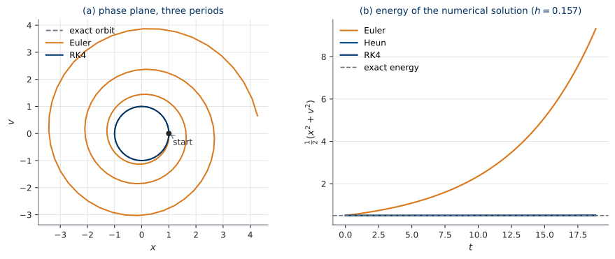
Figure 1 is the emotional anchor of this session, and it is worth being precise about what it does and does not show. It does not show that Euler is unstable in the technical sense; Section 6 defines that word and Euler on this problem sits exactly on the boundary. It shows something more ordinary and more common: a first-order method, applied with a reasonable step size, accumulating a systematic error that a picture makes obvious and a single error number would hide. If you generated images by integrating with this method, you would not see a spiral. You would see samples that are subtly, consistently wrong, and no error message.
The figure is the destination. The animation below is the road, and the road carries the argument. It magnifies the very first step: Euler follows the tangent, lands outside the circle, and the departure is the local error — the \(O(h^2)\) of Equation 3, drawn at a magnification that makes it visible. Nothing about that one step looks alarming, which is exactly why the method is easy to trust. The scene then runs three periods, quarters the step size, and runs them again — the final radius falls from \(4.32\) to \(1.45\), much better and still outside. It closes on Equation 5 with the growth factor measured from the run:
Refinement buys you time, not the property. That is the whole content of the energy law, and it is the reason a smaller step size is not the answer to this picture.
Heun and RK4: buying accuracy with evaluations
Heun: predict, then correct
Euler’s error comes from using the velocity at the start of the step for the whole step. A better estimate would use the average velocity over the step — but the velocity at the end of the step needs the endpoint, which is what you are trying to find.
So guess it. Take an Euler step to get a provisional endpoint, evaluate the field there, and average the two velocities.
\[ \begin{aligned} k_1 &= f(t_n, x_n) , \\ k_2 &= f(t_n + h, \; x_n + h k_1) , \\ x_{n+1} &= x_n + \frac{h}{2} (k_1 + k_2) . \end{aligned} \tag{6}\] Two evaluations of \(f\) per step: 2 NFE per step. The method has order 2.
The prediction \(x_n + hk_1\) is only first-order accurate, and yet the correction it enables is second-order accurate. The reason is that the prediction’s error enters \(k_2\) multiplied by \(h\), so a first-order error in the argument becomes a second-order error in the result. Exercise 1 asks you to verify this by Taylor expansion, and it is the single most instructive calculation on this page.
Heun is also the first appearance of the trade this session is really about: one extra function evaluation per step, in exchange for one extra order. Whether that is a good deal is a question about NFE, and the answer is below.
RK4: the workhorse
The same idea, pushed further. Sample the field at four trial points inside the step, and combine them with weights chosen so that the Taylor expansions cancel to fourth order.
\[ \begin{aligned} k_1 &= f(t_n, \; x_n) , \\ k_2 &= f(t_n + \tfrac{h}{2}, \; x_n + \tfrac{h}{2} k_1) , \\ k_3 &= f(t_n + \tfrac{h}{2}, \; x_n + \tfrac{h}{2} k_2) , \\ k_4 &= f(t_n + h, \; x_n + h k_3) , \\ x_{n+1} &= x_n + \frac{h}{6} \bigl( k_1 + 2 k_2 + 2 k_3 + k_4 \bigr) . \end{aligned} \tag{7}\] Four evaluations of \(f\) per step: 4 NFE per step. The method has order 4.
The weights \(\tfrac{1}{6}, \tfrac{2}{6}, \tfrac{2}{6}, \tfrac{1}{6}\) are Simpson’s rule, and that is not a coincidence: for a right-hand side that does not depend on \(x\) at all, Equation 7 is Simpson’s rule applied to \(\int f(t)\,\mathrm{d}t\).
The Runge–Kutta idea, and where this course stops
Euler, Heun and RK4 are three members of one family. Every member has the same shape: evaluate the field at \(s\) trial points inside the step, each trial point built from the previous evaluations; then combine the evaluations with fixed weights. The coefficients are collected in a table called a Butcher tableau, and the theory of which tableaux achieve which order is a deep and well-developed subject.
This course declines that subject explicitly. We are consumers of tableaux, not designers of them. What you need from the theory is the vocabulary — stage, order, embedded pair — and the three methods above, which cover everything the course does.
The trade, measured
Here is the comparison table, and then the measurement that decides it.
| Method | NFE per step | Order \(p\) | Global error |
|---|---|---|---|
| Euler | 1 | 1 | \(O(h)\) |
| Heun | 2 | 2 | \(O(h^2)\) |
| RK4 | 4 | 4 | \(O(h^4)\) |
Order alone does not settle anything, because a step of RK4 costs four times a step of Euler. The honest comparison is error against NFE, not error against step count.
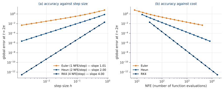
Panel (b) is the answer. Reading a target error of \(10^{-6}\) off the fitted lines, the cost of reaching it on this problem is:
| Method | NFE for a global error of \(10^{-6}\) |
|---|---|
| Euler | \(1.9 \times 10^{7}\) |
| Heun | \(1.3 \times 10^{4}\) |
| RK4 | \(3.8 \times 10^{2}\) |
Two readings of Table 2, and both matter later.
The first is the ordinary one: when accuracy matters and the field is smooth, high order is not a luxury, it is the only affordable option. The second is the caveat: this ordering assumes you want high accuracy. At a loose tolerance the lines in panel (b) are much closer together, and at the extreme — one or two evaluations total — the high-order method has no advantage at all, because it has not taken enough steps for its order to express itself. Sampling a generative model at 4 NFE lives in exactly that regime, and it is why the field’s few-step sampling literature is not simply “use RK4”.
The names on this page reappear as the names of samplers. The sampler of EDM (Karras et al. 2022) is a Heun variant; “Euler sampling” in a diffusion or Flow Matching paper means Equation 3 applied to the learned field \(u_t^\theta\). When U3.T3 discusses them, you will recognise old friends, and you will already know what their NFE per step is.
Adaptive stepping and tolerances
Why a fixed step is the wrong tool
A fixed step size treats every part of the trajectory as equally difficult. Real trajectories are not like that: a solution can be almost straight for most of its length and turn sharply in one short window. A step size small enough for the sharp part wastes evaluations everywhere else, and a step size efficient elsewhere is wrong exactly where it matters.
The fix is to let the solver choose \(h\) as it goes. To do that, it needs to estimate its own error — and it must do so without knowing the exact solution.
Embedded pairs: two orders for almost one price
The trick is to compute the step twice, at two different orders, from the same function evaluations, and to use the difference as an error estimate.
Look again at Heun Equation 6. It evaluates \(k_1\) and \(k_2\). But \(k_1\) alone already gives the Euler step:
\[ \begin{aligned} \hat{x}_{n+1} &= x_n + h k_1 & &(\text{order } 1) , \\ x_{n+1} &= x_n + \tfrac{h}{2}(k_1 + k_2) & &(\text{order } 2) . \end{aligned} \]
Two estimates, one shared evaluation, one extra evaluation total. Their difference estimates the local error of the lower-order one:
\[ \varepsilon_{n+1} \;=\; \bigl\| x_{n+1} - \hat{x}_{n+1} \bigr\| \;=\; O(h^2) . \]
This arrangement is called an embedded pair, written Heun(2)/Euler(1). Every practical adaptive solver is built this way. The value actually propagated is the higher-order one — you paid for it, you may as well keep it — a choice called local extrapolation.
rtol and atol: what the numbers mean
The error estimate \(\varepsilon\) is a vector of absolute numbers, and an absolute number is meaningless on its own: an error of \(10^{-3}\) is negligible if \(x \approx 10^{6}\) and catastrophic if \(x \approx 10^{-6}\). So the estimate is compared against a scale built from two user-supplied tolerances, component by component:
For each component \(i\) of the state, \[ \mathrm{sc}_i \;=\; \texttt{atol} \;+\; \texttt{rtol} \cdot \max\bigl( |x_{n,i}| , \, |x_{n+1,i}| \bigr) , \] and the step is judged by the normalised error \[ \mathrm{err} \;=\; \sqrt{ \frac{1}{d} \sum_{i=1}^{d} \left( \frac{\varepsilon_{n+1,i}}{\mathrm{sc}_i} \right)^{\!2} } . \] The step is accepted when \(\mathrm{err} \le 1\) and rejected otherwise.
Read the scale in its two limits and it explains itself.
rtolis a relative tolerance, and it dominates where the solution is large. Settingrtol\(= 10^{-6}\) asks for roughly six correct significant digits per step.atolis an absolute tolerance, and it dominates where the solution is near zero. Its job is to stop the solver from demanding infinite precision on a component that is passing through zero, where a relative criterion would be unsatisfiable. Set it to the magnitude below which you do not care.
Rejecting a step is not a failure. It is the controller working: the step was computed, judged too inaccurate, thrown away, and retried smaller. Rejected steps cost NFE and produce no progress, which is why a good controller aims to reject rarely.
Whether accepted or rejected, the next step size comes from the same rule. If the local error is \(O(h^{p+1})\), then to hit \(\mathrm{err} = 1\) exactly you would scale \(h\) by \(\mathrm{err}^{-1/(p+1)}\). In practice the rule is damped and clipped:
\[ h_{\text{new}} \;=\; h \cdot \min\!\Bigl( f_{\max} , \; \max\bigl( f_{\min} , \; \; \eta \cdot \mathrm{err}^{-1/(p+1)} \bigr) \Bigr) , \tag{8}\]
with a safety factor \(\eta \approx 0.9\) and clips \(f_{\min} \approx 0.2\), \(f_{\max} \approx 5\). The safety factor makes the next step slightly more conservative than the estimate suggests, so that a marginal step is not immediately rejected. The clips stop a single freak estimate from changing the step size by orders of magnitude.
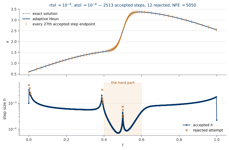
rtol \(=10^{-6}\) and atol \(=10^{-8}\). (a) The computed solution against the exact one, with every 27th accepted step endpoint marked; the ticks crowd together in the transition and thin out elsewhere. (b) The step size against time, log scale, with rejected attempts marked. The solver used \(2513\) accepted steps and \(12\) rejected ones, for a total NFE of \(5050\), and its step size varies by a factor of \(46\) between the easy and the hard part of the same trajectory. It found the hard part without being told where it was.
Figure 3 is the argument for adaptivity in one image. Nobody told the solver that the difficulty was at \(t = 0.5\). The error estimate found it, and the controller responded by spending its evaluations there.
The animation below replays that same run attempt by attempt, from the solver’s own log, and it makes one distinction the figure cannot. Not every rejection means a hard region. The first four rejections happen at small \(t\), where the field is easy; they are the controller leaving \(h_{\text{init}}\) behind and finding its stride. The rejections that follow, four hundred quiet steps later, are the real thing — they arrive at the leading edge of the transition, before its centre, because the error estimate reacts to difficulty as it approaches rather than after it is reached:
The closing summary is the number worth carrying: \(41\%\) of all \(2525\) attempts fall inside \(t \in [0.45, 0.55]\), a window that is a tenth of the interval. The solver concentrated two fifths of its work on a tenth of the problem, and it decided that by itself.
Tolerances too loose. The solver returns quickly, with a small NFE, and a trajectory that looks entirely plausible — smooth, well-behaved, wrong. This is the dangerous failure, because nothing complains. The test is to halve both tolerances and re-run: if the answer moves by more than you can accept, the original answer was not converged.
Tolerances too tight. NFE explodes, the run takes minutes instead of milliseconds, and the extra digits are below the noise of everything else in your pipeline. This is the cheap failure: you notice it immediately, and it costs only time.
The solver you will actually call
The default adaptive solver of scientific computing is RK45, also called Dormand–Prince: an embedded pair of orders 5 and 4, using seven stages of which the last is reused as the first of the next step. It is the default of scipy.integrate.solve_ivp, and the default dopri5 of torchdiffeq and diffrax. When you call an adaptive solver in this course without naming one, this is what runs.
You now know what its arguments mean. That was the point of this section: U2.L1 assumes, without re-explaining, that you know what RK45 and its tolerances do.
With an adaptive solver, NFE becomes data-dependent. The same model, integrated for two different starting points, can cost different amounts. The same model at two different moments of training can cost different amounts.
In U2 you will watch NFE grow during training, and it will hurt. In U3 it stops hurting. Understanding why is a large part of what this course is for.
Stability and stiffness, in pictures
Section 3 measured accuracy as \(h \to 0\). This section is about the opposite question, and it is the one that decides whether a method is usable at all: for a given \(h\), does the numerical solution stay bounded?
The test equation and the stability region
The whole theory is built on one scalar problem, and it earns its place because a linear system can be diagonalised into independent copies of it, one per eigenvalue.
\[ \frac{\mathrm{d}x}{\mathrm{d}t} \;=\; \lambda x , \qquad \lambda \in \mathbb{C} , \qquad x(t) = x_0 e^{\lambda t} . \tag{9}\]
When \(\operatorname{Re}(\lambda) < 0\) the exact solution decays. A numerical method should decay too. Apply Euler to Equation 9:
\[ x_{n+1} = x_n + h \lambda x_n = (1 + h\lambda) \, x_n \quad \Longrightarrow \quad x_n = (1 + h\lambda)^n x_0 . \]
So the numerical solution decays exactly when \(|1 + h\lambda| \le 1\). Every method has such an amplification factor \(R(z)\) with \(z = h\lambda\), and the set where it does not amplify is the method’s stability region.
The region of absolute stability of a one-step method is \[ S \;=\; \bigl\{ \, z = h\lambda \in \mathbb{C} \; : \; |R(z)| \le 1 \, \bigr\} , \] where \(R\) is the factor by which the method multiplies the solution of Equation 9 in one step. For explicit Euler, \(R(z) = 1 + z\); for Heun, \(R(z) = 1 + z + \tfrac{1}{2}z^2\); for RK4, \(R(z) = 1 + z + \tfrac{1}{2}z^2 + \tfrac{1}{6}z^3 + \tfrac{1}{24}z^4\).
Note what \(S\) constrains. It is a condition on the product \(h\lambda\), so it converts a property of the problem, \(\lambda\), into a ceiling on the step size you are allowed to use.
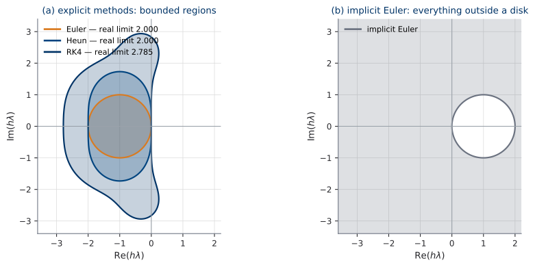
Two readings of Figure 4.
The explicit regions are bounded, and they are all about the same size. RK4 is a thousand times more accurate than Euler at a given \(h\), and its step-size ceiling is only \(39\%\) higher. Order and stability are different currencies, and buying one does not buy the other.
Euler on the harmonic oscillator sits exactly on the boundary. For Equation 4 the eigenvalues are \(\lambda = \pm i\), purely imaginary — and the Euler region touches the imaginary axis only at the origin. So no positive step size is stable for that problem, at all, which is the spiral of Figure 1 now explained. The energy law Equation 5 and the stability region are the same statement twice: \(|1 + ih| = \sqrt{1 + h^2} > 1\) for every \(h > 0\).
Implicit methods, and why this course does not use them
Panel (b) shows the alternative. Implicit Euler is
\[ x_{n+1} \;=\; x_n + h \, f(t_{n+1}, x_{n+1}) , \tag{10}\]
with the unknown on both sides. Its amplification factor is \(R(z) = 1/(1-z)\), so its stability region is the whole complex plane except a disk around \(z=1\) — the entire left half-plane is stable, at any step size.
That property is bought, not given. Each step of Equation 10 requires solving an equation in \(x_{n+1}\), which for a nonlinear \(f\) means an iterative solve with Jacobians. When \(f\) is a neural network, this is expensive in a way that has no counterpart in classical numerical analysis. So the course world is explicit and adaptive, and implicit methods are named here and not implemented.
Stiffness, defined by what it does to you
A problem is stiff on an interval when the step size is limited by stability rather than by accuracy — that is, when a solver is forced to take steps far smaller than the accuracy of the answer would require. The usual cause is a fast decaying mode: a component that dies quickly, stops affecting the answer, and continues to dictate the step size long afterwards.
The definition is operational on purpose. Stiffness is not a property you read off an equation; it is a symptom you observe in a solver.
Here is the symptom, isolated. Take a linear system in two dimensions with one slow mode fixed at \(\lambda_{\text{slow}} = -1\) and one fast mode swept from \(-1\) down to \(-10^{4}\). The fast mode dies almost immediately in every case, so the answer is visually identical every time. The tolerance is identical every time.
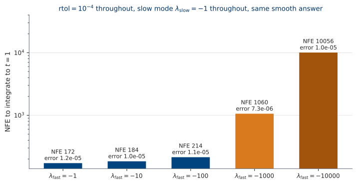
rtol \(=10^{-4}\), as the fast eigenvalue is swept from \(-1\) to \(-10^{4}\) with the slow eigenvalue fixed at \(-1\). Each bar is annotated with the achieved error. The NFE grows by a factor of \(58\); the achieved error does not improve — it stays near \(10^{-5}\) throughout. The extra work does not buy accuracy. It buys stability, for a component of the solution that stopped mattering almost immediately.
Figure 5 is the definition made into a measurement, and the error annotations are the load-bearing part of it. If accuracy had improved with NFE, the figure would show nothing but a solver working harder for a better answer. It did not improve. The work was spent entirely on staying inside the stability region of a mode whose contribution to the answer was already numerically zero.
Are learned velocity fields stiff? It depends on the design, and this course answers the question empirically rather than by assertion: U2.L2 measures the sensitivity of a trained model to solver tolerances, and U3.T4 studies straightness — making the field easy for the solver, so that few steps suffice.
That is the seed worth planting here. A large part of the recent progress in fast sampling is not better solvers. It is fields that are easier to integrate.
The equation that moves the density
One last picture, and one deliberately unanswered question.
Everything above moves a point. But a generative model does not move one point; it moves a whole distribution. You draw many \(x_0\) from the Gaussian, and every one of them follows Equation 1 under the same field. What you care about at \(t=1\) is not any individual trajectory — it is the distribution that the whole cloud has become.
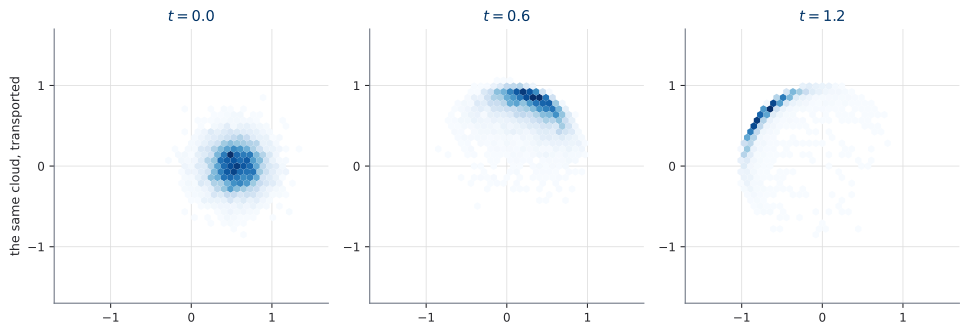
So here is the question. The ODE tells you how a point moves. What equation tells you how the density moves?
There is such an equation, and it is short:
\[ \partial_t \, p_t + \nabla \cdot \bigl( p_t \, u_t \bigr) \;=\; 0 . \]
It is called the continuity equation. It is stated properly and derived in U2.T2, and it becomes the foundation of everything in U3.
Nothing on this page manipulates it. It is here so that you recognise it when it arrives.
One sentence to hold on to until then, and then this session stops: generative modelling in this course means choosing the movie the density should play, and learning the field that plays it.
Exercises, with answers
These are the packet exercises. Work them before reading the answers; the answers are written to be checked against, not read.
Exercise 1 — Heun is order 2
Verify by Taylor expansion that Heun’s method Equation 6 has local truncation error \(O(h^3)\). Work in one dimension and assume \(f\) is as smooth as you need.
Write \(f\) and its derivatives at \((t_n, x_n)\), with \(x_n\) exact. Expand the exact solution: \[ x(t_{n+1}) = x_n + h f + \frac{h^2}{2}\bigl( f_t + f_x f \bigr) + O(h^3) , \] using \(\ddot{x} = \frac{\mathrm{d}}{\mathrm{d}t} f(t, x(t)) = f_t + f_x \dot{x} = f_t + f_x f\).
Now expand the method. The first stage is \(k_1 = f\). The second stage is evaluated at \((t_n + h, \; x_n + hf)\), so a two-variable Taylor expansion gives \[ k_2 = f + h f_t + h f \, f_x + O(h^2) . \] Therefore \[ \begin{aligned} x_n + \frac{h}{2}(k_1 + k_2) &= x_n + \frac{h}{2}\bigl( 2f + h f_t + h f f_x \bigr) + O(h^3) \\ &= x_n + h f + \frac{h^2}{2}\bigl( f_t + f_x f \bigr) + O(h^3) . \end{aligned} \] The \(h\) and \(h^2\) terms match the exact expansion exactly, so the difference is \(O(h^3)\). Local error \(O(h^3)\), global error \(O(h^2)\): order 2.
The point to take away. The prediction \(x_n + hk_1\) is only first-order accurate, and it did not matter — its error entered \(k_2\) multiplied by \(h\), so it landed one order lower than it started.
Exercise 2 — Predict the slopes
You are about to plot the global error of Euler, Heun and RK4 at a fixed final time against the step size \(h\), on log-log axes. Before making the plot: what are the three slopes, and why? Then answer two follow-up questions. (i) What would you see if you plotted against NFE instead of \(h\)? (ii) At what point on the left of the plot would you expect the RK4 line to stop being straight, and why?
The slopes are 1, 2 and 4. Global error \(\approx C h^p\) gives \(\log(\text{error}) = \log C + p \log h\), a straight line of slope \(p\). That is the definition of order, and measuring it is the standard way to confirm that a solver was implemented correctly — a hand-written RK4 that scores slope 3 has a bug, and the slope is what finds it.
(i) Against NFE, the slopes have the same magnitude and the opposite sign, because NFE \(\propto 1/h\) at a fixed method. The lines shift horizontally by the NFE-per-step of each method — Euler by nothing, Heun by a factor of 2, RK4 by a factor of 4 — which is a shift of \(\log 2\) and \(\log 4\), and is small compared with the difference the slopes produce. The ordering therefore survives: see Figure 2(b).
(ii) The RK4 line flattens at the left, at very small \(h\), when the truncation error falls below the floating-point round-off error, which does not shrink with \(h\) and in fact grows slowly as more steps accumulate. In double precision this happens around an error of \(10^{-13}\) or so. Below that you are measuring your arithmetic, not your method.
Exercise 3 — Read a stability region
You must integrate \(\mathrm{d}x/\mathrm{d}t = \lambda x\) with \(\lambda = -50\), from \(t=0\) to \(t=1\), using explicit Euler.
- What is the largest step size that keeps the numerical solution bounded? (b) How many steps is that, at minimum? (c) The exact solution has decayed to \(e^{-50} \approx 2 \times 10^{-22}\) by \(t = 0.5\). Comment on what those steps are buying you after that time. (d) Would switching to RK4 change the picture much?
(a) The stability condition is \(|1 + h\lambda| \le 1\). With \(\lambda = -50\) real and negative, this is \(-2 \le -50h \le 0\), so \(h \le 2/50 = 0.04\).
(b) At least \(1/0.04 = 25\) steps, so at least 25 NFE.
(c) After \(t = 0.5\) the exact solution is smaller than double-precision round-off relative to its initial value; any answer that returns approximately zero is accurate. The steps taken after that point buy no accuracy at all. They are demanded purely by the stability region. This is stiffness, in its smallest possible example: the step size is set by stability, not by the accuracy you need.
(d) Barely. RK4’s real-axis limit is \(2.785\) instead of \(2\), so the ceiling rises to \(h \le 0.0557\) — about 18 steps, at 4 NFE each, so 72 NFE against Euler’s 25. On this problem the higher-order method is worse, because the problem needs stability and RK4 sells accuracy. The real fix for a stiff problem is an implicit method (Equation 10), whose region has no such ceiling.
Exercise 4 — Diagnose the tolerance
For each situation, say whether the tolerances are too loose, too tight, or fine, and say what test would confirm it.
- A run takes 40 seconds and reports NFE \(= 2\,100\,000\); halving both tolerances changes the answer in the eighth decimal place. (b) A run takes 0.2 seconds, reports NFE \(= 30\), and returns a smooth plausible trajectory; halving both tolerances changes the answer in the first decimal place. (c) A run reports 400 accepted steps and 380 rejected ones.
(a) Too tight. The confirming test is the one already described: the answer did not move when the tolerances were halved, so the extra \(10^6\) evaluations bought nothing. Loosen the tolerances until the answer starts to move, then step back one notch.
(b) Too loose, and this is the dangerous case, because the output looked entirely reasonable. The test is the same test, and here it fires: the answer moved in the first decimal place, so the original run was not converged. A plausible-looking trajectory is not evidence of a correct one. Tighten until halving stops changing the answer.
(c) Fine in accuracy, badly configured in control. Rejecting almost half of all attempted steps means the controller is repeatedly overshooting and being pushed back. The accuracy of the accepted steps is not in question — every accepted step passed the test — but roughly half of the NFE was spent on work that was thrown away. Look at the initial step size first, since a wildly wrong \(h_{\text{init}}\) produces a burst of rejections, and then at the safety factor \(\eta\) in Equation 8.
Where each part of this page reappears
| From this session | Reappears in |
|---|---|
f(t, x) time-first convention |
every solver in the course, starting with U0.L5 |
| NFE as a returned output | every solver; the cost axis of U3.L2 and U5 |
| Euler, Heun, RK4 | U0.L5 (implemented by hand); U3.T3 (as sampler names) |
| Adaptive stepping, rtol/atol | U2.L1 (assumed known); U2.L2 (tolerance sensitivity study) |
| Stability and stiffness | U2.L2; U3.T4 (straightness as making fields easy to integrate) |
| The continuity equation | U2.T2 (derived); U3.T1 (the foundation of Flow Matching) |
Optional reading
For the curious, and not required: (Kidger 2022) covers numerical ODE solvers with neural differential equations in view throughout, which is the combination this course is heading towards. The standing textbook reference for the unit is (Bishop and Bishop 2024).
Next session
The next lab session (U0.L5) implements everything on this page from scratch: Euler, Heun, RK4 and one adaptive method, each returning its NFE; then the log-log plot of Figure 2, made by you, with the slopes you predicted in Exercise 2. After that, the same toy problem in JAX.