U0.T5 — Numerical ODE Solvers

Flow-Based Generative Models · UFRJ · 2026.2

01Why solvers, why now

From U2 on, sampling is solving

\[ \frac{\mathrm{d}x}{\mathrm{d}t} \;=\; u_t(x) , \qquad x(0) = x_0 \sim \mathcal{N}(0, I_d) \]

Draw noise at \(t=0\). Follow the field. Whatever you reach at \(t=1\) is your sample.

The network is the right-hand side. Today is about everything to the left of the equals sign.

Callback to the U0.T4 signature board: the network (x, t) → ẋ is exactly f in an IVP. Point at it. Today we never train anything — this is classical numerical analysis, and it would read the same in 1960.

The word for the whole session

NFE = number of function evaluations: how many times a solver calls \(f\) while integrating.

\[ \text{cost of one sample} \;=\; \text{NFE} \times (\text{one forward pass}) \]

Every evaluation of \(u_t^\theta\) is a forward pass through a neural network.

By December you will discuss papers whose entire contribution is reducing NFE.

Say the number out loud: a 1000-step sampler is 1000 forward passes per image. That is why NFE is the currency.

02Euler and the anatomy of error

The problem, and the convention

\[ \frac{\mathrm{d}x}{\mathrm{d}t} = f(t, x(t)) , \qquad x(t_0) = x_0 \]

Right-hand sides are f(t, x) — time first. Every solver returns its NFE.

Existence and uniqueness need \(f\) Lipschitz in \(x\) — that is Picard–Lindelöf, stated properly in U2.T1.

f(t,x) matches solve_ivp, torchdiffeq and diffrax. Argument order is exactly the convention that costs an afternoon when found late: f(x,t) runs, converges, and is wrong.

Euler: follow the tangent

At \(x_n\) the equation gives you the velocity. Pretend it holds for a time \(h\).

\[ x_{n+1} = x_n + h \, f(t_n, x_n) \qquad \textbf{1 NFE per step} \]

A polygon inscribed in a curve.

Board 1 starts here and stays up through block C. Draw the curve, draw one tangent step, draw the gap.

Two errors, not one

The error of one step, started from the exact point: \[ \tau_{n+1} = x(t_{n+1}) - \bigl[\, x(t_n) + h f(t_n, x(t_n)) \,\bigr] \]

The error that actually reaches you, after all \(N\) steps: \[ e_N = x(t_N) - x_N \]

Order \(p\): local \(O(h^{p+1})\), global \(O(h^{p})\). One power is lost to accumulation.

This distinction is where self-studiers stumble — the notes work it much more slowly. The bookkeeping in one line: N ≈ 1/h steps, each contributing h^(p+1), gives h^p.

The proof, part 1: local error is \(O(h^2)\)

Taylor-expand the exact solution about \(t_n\):

\[ x(t_{n+1}) = x(t_n) + h \, \dot{x}(t_n) + \frac{h^2}{2}\ddot{x}(\xi) \]

The ODE says \(\dot{x}(t_n) = f(t_n, x(t_n))\) — the first two terms are the Euler step.

\[ \Longrightarrow \quad \tau_{n+1} = \frac{h^2}{2}\,\ddot{x}(\xi) \;=\; O(h^2) \]

Board 1. Three lines, do them live and slowly. Stress that the Euler step here starts from the EXACT point — that is what makes it local.

The proof, part 2: accumulation costs one power

Let \(e_n = x(t_n) - x_n\). Subtract the two updates and take norms:

\[ \|e_{n+1}\| \;\le\; (1 + hL)\,\|e_n\| \;+\; \tfrac{1}{2} M h^2 \]

\(L\) = Lipschitz constant of \(f\) in \(x\). Unroll from \(e_0 = 0\):

\[ \|e_N\| \;\le\; \frac{Mh}{2L}\Bigl[\, e^{L(t_1 - t_0)} - 1 \,\Bigr] \;=\; O(h) \]

Read the constant: it grows like \(e^{L(t_1-t_0)}\). Order 1 is a statement about a slope, not a promise of a small number.

Keep Board 1 up. The exponential constant is the honest part and it sets up block E: when hL stops being small, “order 1” tells you nothing useful.

The picture to keep

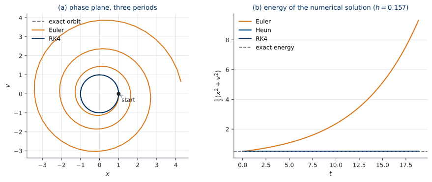
Explicit Euler on the harmonic oscillator, \(h = 2\pi/40\). Left: three periods in the phase plane — the exact orbit is the unit circle; Euler ends at radius \(4.32\). Right: energy against time.

\[ E_{n+1} = \tfrac12\bigl[(x_n + hv_n)^2 + (v_n - hx_n)^2\bigr] = (1 + h^2)\,E_n \quad \textbf{exactly} \]

Not a plotting artifact — the cross terms cancel and the growth factor is exact, at every h. Smaller h slows the spiral; no h stops it. Ask: if you generated images this way, what would you see? Answer: not a spiral — samples that are quietly, consistently wrong, with no error message.

The same picture, one step at a time

The static figure is the destination. This is the road, and the road is where the argument lives.

Two beats are the ones to wait for. The first step is magnified: it follows the tangent, it lands outside the circle, and the departure is the local error. Nothing about that first step looks alarming — that is the point.

Then the scene quarters the step size and runs it again. The radius after three periods goes from 4.32 to 1.45. Much better, still outside. Say plainly what that means: refinement buys you time, not the property. The energy law on the previous slide is why.

03Heun and RK4

Heun: predict, then correct

Euler uses the velocity at the start for the whole step. Average the two ends instead — and guess the far end with Euler.

\[ \begin{aligned} k_1 &= f(t_n, x_n) , \qquad k_2 = f(t_n + h, \; x_n + h k_1) \\ x_{n+1} &= x_n + \tfrac{h}{2}(k_1 + k_2) \qquad \textbf{2 NFE per step, order 2} \end{aligned} \]

The first NFE-vs-accuracy trade of the course: one extra evaluation, one extra order.

Why does a first-order prediction give a second-order method? Because the prediction’s error enters k2 multiplied by h. That is Exercise 1 in the notes — the single most instructive calculation on the page.

RK4: the workhorse default

\[ \begin{aligned} k_1 &= f(t_n, \, x_n) , &\quad k_2 &= f(t_n + \tfrac{h}{2}, \; x_n + \tfrac{h}{2}k_1) , \\ k_3 &= f(t_n + \tfrac{h}{2}, \; x_n + \tfrac{h}{2}k_2) , &\quad k_4 &= f(t_n + h, \; x_n + h k_3) , \\ x_{n+1} &= x_n + \tfrac{h}{6}\bigl(k_1 + 2k_2 + 2k_3 + k_4\bigr) . & &\textbf{4 NFE, order 4} \end{aligned} \]

The weights \(\tfrac16, \tfrac26, \tfrac26, \tfrac16\) are Simpson’s rule — and for an \(f\) that does not depend on \(x\), RK4 is Simpson’s rule.

Shown, not derived. If someone asks where the coefficients come from: Butcher theory, next slide, and we are declining it on purpose.

The Runge–Kutta idea, and where we stop

The idea, in one sentence: sample the field at trial points inside the step, then combine the samples with fixed weights so the Taylor terms cancel.

The coefficients live in a Butcher tableau. The theory of which tableaux reach which order is deep, well developed, and explicitly declined here.

We are consumers of tableaux, not designers of them.

You need three methods and three words: stage, order, embedded pair.

Order and cost

Method	NFE / step	Order \(p\)	Global error
Euler	1	1	\(O(h)\)
Heun	2	2	\(O(h^2)\)
RK4	4	4	\(O(h^4)\)

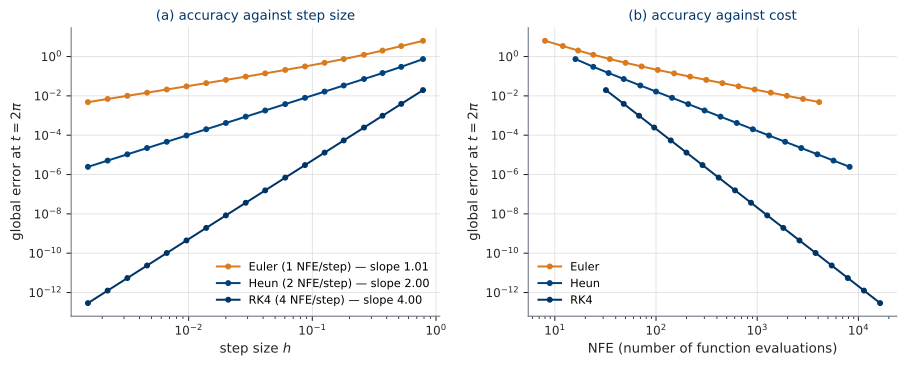
Order alone settles nothing: an RK4 step costs four Euler steps.

The honest axis is NFE, not step count.

Next slide is the measurement. Students make this plot themselves in U0.L5 — ask them now to predict the three slopes before they see it.

Error against \(h\), and against cost

Global error at \(t = 2\pi\). Left: against step size, log-log — fitted slopes \(1.01\), \(2.00\), \(4.00\). Right: the same errors against NFE, the honest cost axis.

NFE to reach a global error of \(10^{-6}\): Euler \(1.9\times10^{7}\) · Heun \(1.3\times10^{4}\) · RK4 \(3.8\times10^{2}\)

Five orders of magnitude. But state the caveat: this ordering assumes you want HIGH accuracy. At 4 NFE total, RK4 has no advantage — it has not taken enough steps for its order to express itself. That regime is exactly where few-step samplers live, and it is why “just use RK4” is not the answer in U3.

Why this matters later

The names on this slide come back as the names of samplers.

“Euler sampling” in a diffusion or Flow Matching paper means exactly \(x_{n+1} = x_n + h\,u_{t_n}^\theta(x_n)\). The EDM sampler is a Heun variant.

When U3.T3 discusses them, you will recognise old friends — and you will already know their NFE per step.

04Adaptive stepping and tolerances

A fixed step is the wrong tool

A trajectory can be almost straight for most of its length and turn sharply in one short window.

• A step small enough for the sharp part wastes evaluations everywhere else.
• A step efficient elsewhere is wrong exactly where it matters.

So let the solver choose \(h\) as it goes — which means it must estimate its own error, without knowing the answer.

Embedded pairs: two orders, one extra evaluation

Heun already computes \(k_1\) and \(k_2\). But \(k_1\) alone is the Euler step:

\[ \hat{x}_{n+1} = x_n + h k_1 \;\; (\text{order }1) , \qquad x_{n+1} = x_n + \tfrac{h}{2}(k_1 + k_2) \;\; (\text{order }2) \]

\[ \varepsilon_{n+1} = \bigl\| x_{n+1} - \hat{x}_{n+1} \bigr\| \;=\; \text{local error estimate} \]

Written Heun(2)/Euler(1). Propagate the higher order — you paid for it.

Board 2 starts here: the accept/reject loop as a flowchart. Every practical adaptive solver is built exactly this way.

What rtol and atol actually mean

\[ \mathrm{sc}_i = \texttt{atol} + \texttt{rtol}\cdot\max\bigl(|x_{n,i}|,\,|x_{n+1,i}|\bigr) , \qquad \mathrm{err} = \sqrt{\frac{1}{d}\sum_i \Bigl(\frac{\varepsilon_{n+1,i}}{\mathrm{sc}_i}\Bigr)^{\!2}} \] Accept the step when \(\mathrm{err} \le 1\). Otherwise throw it away and retry smaller.

• rtol dominates where \(x\) is large — it asks for significant digits.
• atol dominates where \(x\) is near zero — it says how small is “don’t care”.

Without atol, a component crossing zero would demand infinite precision for a reason that has nothing to do with the field. Board 2: draw the scale as a tube around the trajectory that narrows where x is small.

The step-size controller

\[ h_{\text{new}} \;=\; h \cdot \min\Bigl( f_{\max} , \; \max\bigl( f_{\min} , \; \eta \cdot \mathrm{err}^{-1/(p+1)} \bigr) \Bigr) \]

• The exponent \(-1/(p+1)\) is just “solve \(\mathrm{err} = 1\)” for the local order \(p\).
• \(\eta \approx 0.9\) — a safety factor, so a marginal step is not immediately rejected.
• \(f_{\min}\approx 0.2\), \(f_{\max}\approx 5\) — clips, so one freak estimate cannot change \(h\) by orders of magnitude.

A rejected step is the controller working, not failing. It still costs NFE.

The solver finds the hard part by itself

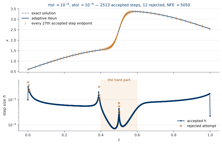
Embedded Heun(2)/Euler(1), rtol \(=10^{-6}\), atol \(=10^{-8}\). Top: solution with every 27th accepted step endpoint marked. Bottom: step size against time, log scale, rejected attempts marked.

\(2513\) accepted, \(12\) rejected, NFE \(= 5050\); step size varies by a factor of \(46\) along one trajectory.

Nobody told it the difficulty was at t = 0.5. The error estimate found it and the controller spent the evaluations there. That is the whole argument for adaptivity.

The hunt, played from the attempt log

This is the same run as the figure, replayed attempt by attempt from its own log — not a re-enactment.

One nuance the static figure cannot give, and it is worth the slide on its own: the first four rejections are not difficulty. They are the controller leaving h_init behind. Students read every rejection as a hard region, and this run shows two different causes for the same symptom.

Then four hundred quiet steps, then err jumps well over 1 at the leading edge of the transition — before its centre. Close on the summary: 41 % of all attempts fall inside t in [0.45, 0.55], a window that is a tenth of the interval. And 12 rejections in 2525 attempts, which is what a controller that is working looks like.

Two failure smells

Fast, small NFE, a smooth plausible trajectory that is wrong. Nothing complains.

Test: halve both tolerances and re-run. If the answer moves, it was never converged.

NFE explodes; the extra digits are below the noise of everything else. You notice immediately.

Same test diagnoses both — that is why it is worth memorising. Exercise 4 in the notes is three cases of this.

The solver you will actually call

RK45, also called Dormand–Prince: an embedded pair of orders 5 and 4, seven stages.

• the default of scipy.integrate.solve_ivp
• dopri5 in torchdiffeq and in diffrax

You now know what every one of its arguments means.

With an adaptive solver, NFE becomes data-dependent. In U2 you will watch it grow during training, and it will hurt. In U3 it stops hurting. Understanding why is the course.

The gray line is a forward flag with no punchline today. Do not explain why it stops hurting — that is U3.

05Stability and stiffness

The other question about \(h\)

Block B asked: how accurate is this as \(h \to 0\)?

Block E asks the question that decides whether a method is usable at all:

For a given \(h\), does the numerical solution stay bounded?

Test equation — a scalar problem, because a linear system diagonalises into copies of it:

\[ \frac{\mathrm{d}x}{\mathrm{d}t} = \lambda x , \quad \lambda \in \mathbb{C} , \qquad x(t) = x_0 e^{\lambda t} \]

Amplification, and the region

Euler on the test equation:

\[ x_{n+1} = (1 + h\lambda)\,x_n \quad \Longrightarrow \quad x_n = (1+h\lambda)^n x_0 \]

\[ S = \bigl\{\, z = h\lambda \in \mathbb{C} \;:\; |R(z)| \le 1 \,\bigr\} \] Euler \(R(z) = 1+z\); Heun \(R(z) = 1 + z + \tfrac{z^2}{2}\); RK4 through \(\tfrac{z^4}{24}\).

\(S\) constrains the product \(h\lambda\) — so it is a ceiling on your step size.

Board 3: draw the complex hλ plane large, and keep it up for the rest of the block.

The regions

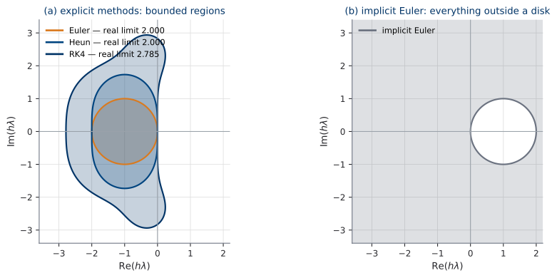
Shaded = stable. Left: the explicit methods, all bounded; real-axis limits \(2.000\), \(2.000\), \(2.785\), located by bisection. Right: implicit Euler — everything outside a disk.

RK4 is \(10^3\times\) more accurate than Euler at a given \(h\), and its step ceiling is only \(39\%\) higher. Order and stability are different currencies.

The spiral, explained

The harmonic oscillator has eigenvalues \(\lambda = \pm i\) — purely imaginary.

The Euler region touches the imaginary axis only at the origin. So:

\[ |1 + ih| = \sqrt{1 + h^2} \; > \; 1 \quad \text{for every } h > 0 \]

No positive step size is stable for that problem. The energy law and the stability region are the same statement twice.

Point back at the block B figure. This is the payoff of keeping it up.

Implicit methods, named and declined

\[ x_{n+1} = x_n + h\,f(t_{n+1},\, x_{n+1}) \qquad \text{(unknown on both sides)} \]

\(R(z) = 1/(1-z)\) — the whole left half-plane is stable, at any step size.

That is bought, not given: each step solves an equation in \(x_{n+1}\), which for a nonlinear \(f\) means an iterative solve with Jacobians.

Our fields are expensive neural networks. The course world is explicit + adaptive; implicit solvers are named here and never implemented.

Stiffness, defined by the symptom

A problem is stiff when the step size is limited by stability rather than by accuracy — the solver is forced far below the step the answer needs.

Usual cause: a fast decaying mode that dies quickly, stops affecting the answer, and keeps dictating \(h\) long afterwards.

Not a property you read off an equation. A symptom you observe in a solver.

Stiffness, measured

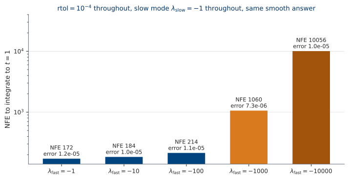
NFE to integrate a 2D linear system to \(t=1\) at rtol \(=10^{-4}\); slow mode fixed at \(-1\), fast mode swept to \(-10^{4}\). Each bar is annotated with the achieved error.

NFE grows \(58\times\). The error does not improve — it sits near \(10^{-5}\) throughout.

The error annotations are the load-bearing part. If accuracy had improved, this would just be a solver working harder for a better answer. It did not. The work bought stability for a component that was already numerically zero.

An honest scope note

Are learned velocity fields stiff? It depends on the design, and this course answers it empirically, not by assertion:

• U2.L2 — tolerance-sensitivity study on a trained model
• U3.T4 — straightness: making the field easy to integrate

A large part of recent progress in fast sampling is not better solvers. It is fields that are easier to integrate.

06The equation that moves the density

One field, a whole cloud

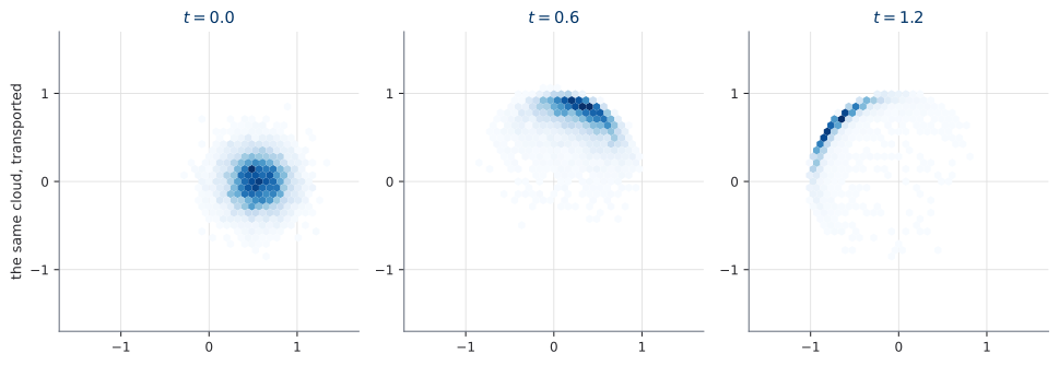
One cloud of initial conditions, transported by a single velocity field, at three times. Every point obeys the same ODE. Nobody moves the cloud as a whole — and yet the density changes shape.

The ODE moves a point. What moves the density?

Pose the question and let it sit. Do not answer it. This slide is the teaser and the next one shows the equation grayed — shown, never manipulated.

Shown, not derived

\[ \partial_t \, p_t + \nabla\cdot\bigl(p_t \, u_t\bigr) = 0 \]

The continuity equation. Stated properly and derived in U2.T2. It becomes the foundation of everything in U3.T1.

Generative modelling in this course = choosing the density movie, and learning the field that plays it.

Gray-teaser protocol: do NOT manipulate this equation, do not derive it, do not integrate it against a test function. If someone pushes: “U2.T2”. Then stop and move to the close.

07Close

What this session hands forward

From today	Reappears in
f(t, x) time first; NFE returned	every solver, from U0.L5 on
Euler, Heun, RK4	U0.L5 (by hand); U3.T3 (as samplers)
Adaptive stepping, rtol/atol	U2.L1 (assumed); U2.L2
Stability and stiffness	U2.L2; U3.T4 (straightness)
The continuity equation	U2.T2 (derived); U3.T1

These notes are the PESC packet

The lecture notes for this session are written standalone-first: complete prose, self-explanatory figures, exercises with answers, everything runs on CPU.

They are the core of the self-study packet PESC students receive at enrollment — which makes them your best review document too.

Next session (U0.L5): implement all four solvers from scratch, each returning its NFE; make the log-log plot yourself; then the same toy ODE in JAX.

Say the packet framing out loud — PGMAT students should know why these notes are written differently from the others, and that the difference is in their favour. Predict the slopes before the next session.