U0.L4 — U-Net Skeleton and Eval Harness

Flow-Based Generative Models · UFRJ · 2026.2

01The contracts

Today you freeze two interfaces

Every previous lab ended by freezing an interface. This one starts by freezing two, because the freeze is the deliverable.

• unet-skeleton — U3.L2 trains it, U3.L3 conditions it, PS0 imports it
• eval-harness — every number this course reports, from here on

The primitive blocks are given to you complete. You write the wiring, the conditioning path, and the metrics — the parts that transfer.

Two minutes. The framing that has to land: today’s output is not a result, it is infrastructure. Four later sessions import these names. Say plainly that the scaffolding is higher than usual and why: transcribing conv boilerplate under time pressure teaches nothing, and these artifacts have to be correct because everything else sits on them.

The unet-skeleton contract — frozen

UNet(in_ch, base_ch, ch_mults,
     attn_resolutions, num_classes=None)

forward(x: (B,C,H,W) float,
        t: (B,)      float in [0,1],
        y: (B,)      long, optional) -> (B,C,H,W)

1. t is always (B,) floats in \([0,1]\) — the FM arrow in code
2. y optional; the label embedding is summed into \(\mathrm{emb}(t)\)
3. output has the input’s shape

Read the three laws off the slide. Do not elaborate yet — the next slide is the elaboration of law 1, which is the one that matters.

Law 1 is what keeps the dialect out

Every reference implementation you will read takes an integer timestep counting down from a thousand.

Every one of them therefore invites \(\beta_t\), \(\bar\alpha_t\) and a reversed arrow into your code — one function at a time, until the codebase speaks two languages.

The assert in forward refuses the first step of that.

Any later code needing another time variable converts outside the network.

This is the slide to slow down on. The point is not notational fussiness: it is that a codebase with two time conventions produces bugs that look like modelling errors. Ask them where they have seen 1 - t appear twice.

The eval-harness contract — frozen

FeatureExtractor        # name, preprocessing, dim
  MNISTFeatures         # pinned course classifier
  InceptionV3Features   # CIFAR and beyond

ref_stats(loader, extractor) -> RefStats
fid(samples, ref, extractor) -> float
bpd(mean_log_lik_nats, num_dims) -> float
panel(sample_fn, eps_bank, path) -> figure

The comparability rule: an FID is a property of a model and a measurement protocol.

Point at the rule and say it will be enforced by the code rather than by memory — that comes back in Part D.

Caveat (iii), settled for this course

U0.T4 left it open: the extractor decides what “similar” means.

MNIST → MNISTFeatures: a small CNN trained on MNIST, weights pinned and committed, penultimate layer (128 units).

Inception is reserved for CIFAR and beyond.

The weights are pinned, not trained by you — every FID in this course must be comparable across students and machines, which needs one shared feature space.

Show the pinned accuracy: 99.22% on ten thousand held-out images, seed 0, best-on-val selection, SHA recorded beside it. Then the twist: running the training script again gives a different extractor and therefore a different, self-consistent, incomparable scale. That is caveat (i) one level up.

One deliberate inconsistency, named

The extractor uses BatchNorm. The recipe card bans BatchNorm from the U-Net.

The law is about the failure, not about the layer.

• A generative model is sampled one at a time → batch statistics would make one sample depend on the others
• A classifier used only in eval() runs on frozen running statistics → depends on no batch at all

Someone always spots this, and it is better to spot it for them. The general lesson is worth stating: a rule you can only apply by memorising the layer name is a rule you will misapply.

02Assembling the U-Net

The build map

The diagram is U0.T4’s, unchanged (Ronneberger, Fischer, and Brox 2015). Every box in it is something you wire today.

Leave this up through the whole assembly part. Point at the dashed arcs and remind them: concatenation, not addition.

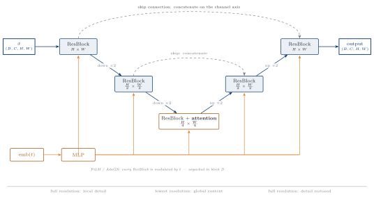
TODO 1 — the ladder, frozen at U0.T4

half  = dim // 2
freqs = torch.exp(-math.log(10000.0)
                  * torch.arange(half) / half)
arg   = (1000.0 * t)[:, None] * freqs[None, :]
emb   = torch.cat([sin(arg), cos(arg)], dim=-1)

The factor \(1000\) is the only rescale, and it is deliberate: it makes this ladder produce the same numbers as DiT and ADM.

So a later cross-check against a library reports a real bug, not a convention difference.

Emphasise: outside this one function, t is a float in [0,1] everywhere. The 1000 lives inside the embedding and nowhere else.

TODO 2 — the wiring, and the shape table

The honest difficulty of the session, and it is bookkeeping.

Level	Resolution	Channels	Attention
0	\(28 \times 28\)	64	—
1	\(14 \times 14\)	128	—
2	\(7 \times 7\)	128	yes
bottleneck	\(7 \times 7\)	128	yes

Attention only at the bottom: cost is quadratic in positions, so \(7\times7\) costs about \(1/256\) of \(28\times28\).

Write the skip stack on the board as a literal stack: push on the way down, pop on the way up. The channel count of what you pop is what decides the decoder block’s input width.

The one-extra-block rule

The decoder gets one more residual block per level than the encoder.

Not style. The level’s last skip is the one the downsampling layer pushed, and it needs a block of its own to be consumed.

A decoder with matching block counts leaves one skip on the stack — and the failure is a shape error deep inside the last level, not anything legible.

This is the single place most students lose fifteen minutes. Say the symptom out loud so they recognise it: a channel-count mismatch in the last decoder block usually means the block count, not the multipliers.

The stack, filling and draining

The scene runs the ladder twice. First correctly: the encoder pushes, the decoder pops in reverse order, and the stack ends empty. Then with the encoder’s block count, in orange.

Be precise about how the second run fails, because the scene is. It does not run to the end and leave a tile over. It stops early, at a pop where the decoder is at one resolution and the tile is at another — the missing block is the one that upsamples. The shortfall count that follows is marked on screen as a counterfactual, and it is one tile per level, not one in total.

The arc diagram of U0.T4 cannot show any of this, because a count going wrong is a fact about time, not about wiring.

TODO 3 — the conditioning path

\[ c = \mathrm{emb}(t) + \mathrm{emb}(y) \;\longrightarrow\; \text{MLP} \;\longrightarrow\; (\gamma, \beta) \]

The modulation itself is FiLM (Perez et al. 2018). What is new here is the sum: the label table has the ladder’s width, not d_emb, so the sum happens before the projection.

One projection, whatever the number of signals. Concatenating would grow the modulation path every time a signal was added, and need a wider projection in every block.

Tie back to U0.T4’s embedding-sum rule. The price of the class pathway is on the next slide and it is tiny, which is the argument for building it today.

Checkpoint — three things pass

1. Shapes — \(28\times28\) in, \(28\times28\) out; and again at \(14\times14\)
2. Parameters within 5 %: 6 946 881, or 6 947 521 with ten classes
3. The reading question — the blocks call num_groups(channels), not 32. What does it give for 64, 128 and 1?

The class pathway costs 640 parameters: ten vectors of width 64. That is the whole price of building it a unit early.

Answer to the reading question: GroupNorm needs the group count to divide the channel count, so hard-coding 32 crashes as soon as base_ch is not a multiple of it. num_groups returns 32, 32 and 1.

03Is the conditioning alive?

The plan for this part contradicted itself

Two checks the session plan asked for, in this order:

• Ritual 1 — fix \(x\), sweep \(t\), assert the outputs differ
• Ritual 2 — at init, assert the output is zero

Run both at initialization and they cannot both hold.

Zero-init does not make the output approximately zero. It makes it exactly zero, for every \(t\) — so ritual 1 must fail, and not because anything is broken.

Let this land before showing the figure. Ask them which of the two rituals they would drop; the answer is neither, and the fix is ordering.

Measured

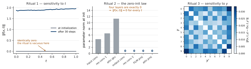
The flat grey line is not dead conditioning. It is a network that is the zero function — exactly what ritual 2 demands.

Left panel is the finding. Middle: four norms, all exactly zero, on a log axis. Right: the ten-by-ten label distance matrix — note it is not near-constant, which is what an embedding table should give you.

The rule that comes out of it

A check that asserts a network does something cannot run at initialization, if the initialization is designed to make the network do nothing.

Zero-init check first, at init. Then move the parameters. Then everything else.

Second time this course has met this shape — U0.L3’s gradient check had the same defect, for the same reason.

Recall U0.L3 explicitly: with zero-init heads the gradient into the encoder body is exactly zero, so the check reported a perfect 0.0 relative error while measuring nothing. Two instances is a pattern worth naming.

Moving the parameters is not training

Thirty optimizer steps against random targets. No dataset, no generative objective, result discarded.

x, t, target = randn(8,1,28,28), rand(8), randn(...)
loss = ((model(x, t) - target) ** 2).mean()

The U-Net is not trained today. Its first real training is U3.L2, by design.

Be explicit that this is a deliberate boundary, not an oversight. They will ask why they cannot train it now; the answer is that training it needs an objective the course has not built yet.

The three rituals, and what each catches

Ritual	Asserts	Catches
\(t\) sensitivity	outputs differ over \(t\)	a conditioning path wired to nothing
zero-init	output exactly \(0\) at init	a lost zero-init
\(y\) sensitivity	outputs differ over \(y\)	a dead class pathway
gradient check	finite diff = autograd	a wrong hand-written derivative

A conditioning path wired to nothing still trains, the loss still falls, and the model is a \(t\)-independent average.

That last sentence is the reason the rituals exist. Silent failure, plausible loss curve, useless model. Also mention the self-test: the gradient check is re-run against a deliberately doubled gradient and must fail there. If someone asks for the ritual numbers: about 5.6% relative spread over t, label distances from 0.004 to 0.034, gradient relative error of order 1e-7 — and say they move in the last digits between runs, because GPU determinism is opt-in and a seed alone does not buy it.

04The evaluation harness

TODO 4 — why float64, and why the filename

float64 accumulation is not fastidiousness. A covariance sums products across orders of magnitude; in float32 the small terms are lost, and the matrix can fail to be positive semi-definite.

The failure then surfaces two functions away, as a complex number nobody expected.

refstats__mnist-test__mnist-cnn-v1__01-float-28x28.npz

A key without the preprocessing serves the wrong pipeline on a hit — silently, permanently.

The filename slide is worth a beat. Making a rule impossible to violate beats writing it in a docstring, and this is the cheapest example of that they will see all semester.

TODO 5 — the square root, and the wrong fix

\[ \mathrm{FID} = \lVert \mu_r - \mu_g \rVert^2 + \operatorname{Tr}\!\big( \Sigma_r + \Sigma_g - 2 (\Sigma_r \Sigma_g)^{1/2} \big) \]

sqrtm returns a complex array. The true root is real; floating point decorates it with a tiny imaginary part.

The standard fix — call .real — is wrong, and only sometimes. A large imaginary part means the input was not PSD: a real bug upstream. So: measure before truncating.

Show the guard in the code. The general habit: when you discard something, check the size of what you discard.

Caveat (i), made unavoidable

fid returns a FIDValue — it is a float, and it carries its protocol.

>>> a = fid(...)   # n = 2000
>>> b = fid(...)   # n = 10000
>>> a.check_comparable(b)
ValueError: not comparable — caveat (i).

A docstring warning does not survive contact with a results table, where two numbers sit in one column with nothing to say how each was measured.

Recall the U0.T4 measurement: score a genuinely better model with fewer samples than its rival and it loses in every one of 40 trials.

TODO 6 and 7 — bits per dimension, and the panel

\[ \mathrm{BPD} = -\frac{\mathbb{E}_{x \sim q}[\log p_\theta(x)]}{d \log 2} \]

Mechanical today. The dequantization term is deliberately absent — it is added when U1 first uses this number, and the docstring says so in as many words.

panel formalizes U0.L3’s trick: a fixed noise bank, so two panels differ because the model changed and not because the noise did.

On the missing term: the marker in the docstring is the point. An absence nobody recorded is indistinguishable from a decision nobody made.

05Calibrating the instrument

Three cases whose answer is known

A metric is not trusted because it is implemented. It is trusted because it was checked. FID (Heusel et al. 2017) is no exception.

1. Split test — MNIST cut in half; true FID is exactly zero
2. Sample-count curve — the same split at several \(n\)
3. Garbage test — noise images against MNIST

These three numbers go in every student’s session log.

Frame it as instrument calibration, because that is what it is. You would not trust a thermometer you had never put in ice water.

The bias is real, and it is a law

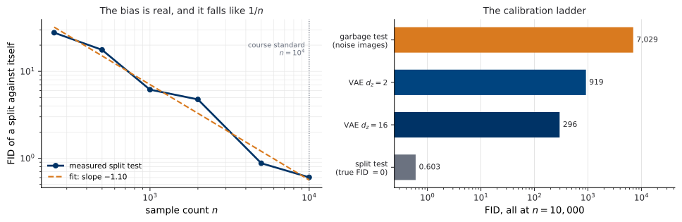
Report at a fixed sample count — ten thousand for MNIST — or report the whole curve. Never compare across counts.

Left panel: six counts, monotone, fitted log-log slope minus 1.10; the points scatter around the line because each count is one draw, not an average. Right panel: the split test is 0.603 and the garbage test is 7028.6 — a factor of eleven thousand, which is the dynamic range of the instrument.

The payoff — the eye test becomes a number

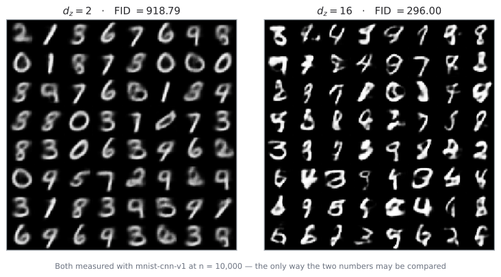
In U0.L3 the wider VAE “looked better”. Now it has a size.

This is the emotional beat of the session: the first real generative evaluation of the course, on their own model from two sessions ago. Read both numbers — 918.8 at d_z = 2 against 296.0 at d_z = 16, a factor of 3.1 — and stress that they were measured at the same n with the same extractor, which is the only reason they may be put side by side. Warn them off the absolute scale: 128 unnormalised units from a small MNIST classifier is not comparable with any published Inception-based MNIST FID.

One preprocessing decision inside that number

The VAE decoder outputs Bernoulli probabilities. Its samples could be those, or binary draws from them.

The reference side is grayscale MNIST, and the extractor’s preprocessing is named 01-float-28x28.

Thresholding would compare a binary set against a grayscale one — a protocol mismatch, on the reference side, invisible in the resulting number.

So the harness scores the probabilities.

Exactly the class of thing caveat (i) is about, and the reason the extractor carries a preprocessing string at all. Ask them where else in the pipeline this decision could hide.

06The freeze

Both artifacts are frozen

Tagged u0l4-freeze. From here a change to either interface is a breaking change and needs a dated CHANGELOG note.

This is not an exercise. U3.L2 imports UNet and trains it. U3.L3 switches on the class pathway. U1.L2 imports bpd. PS0 imports everything.

Extend without breaking: add keyword-only arguments with defaults, never change the positional contract — the hygiene-stack lesson, applied to a second artifact.

UNet already carries three keyword-only extras and every call against the frozen five-argument form still works. That is the demonstration.

PS0 is assembled

Component	Built in	Role
vae-mnist-scratch	U0.L3	the base codebase
unet-skeleton	here	replaces the encoder
hygiene-stack	U0.L2	the training discipline
eval-harness	here	the numbers and the panels

Graded on correctness and reproducibility — config, seed, commit, tracking database — not on sample quality.

Draft statement visible today; formally assigned at the end of U0.L5.

Show the draft statement briefly. They have now built every part of PS0 and it is worth saying so.

Next session (U0.T5): the last drawer

Numerical solvers for ordinary differential equations — the drawer the second half of this course lives in.

Every continuous-time model from U2 on is defined by a velocity field and realized by a solver. The number of function evaluations becomes a reported quantity beside the quality of what it produced.

The instrument you calibrated today is what makes that trade measurable — U3.L2 plots function evaluations against FID, on the network you assembled today.

Close on the connection. Today felt like infrastructure; the exit line says where the infrastructure is spent.

References

Heusel, Martin, Hubert Ramsauer, Thomas Unterthiner, Bernhard Nessler, and Sepp Hochreiter. 2017. “GANs Trained by a Two Time-Scale Update Rule Converge to a Local Nash Equilibrium.” In Advances in Neural Information Processing Systems. https://arxiv.org/abs/1706.08500.

Perez, Ethan, Florian Strub, Harm de Vries, Vincent Dumoulin, and Aaron Courville. 2018. “FiLM: Visual Reasoning with a General Conditioning Layer.” In AAAI Conference on Artificial Intelligence. https://arxiv.org/abs/1709.07871.

Ronneberger, Olaf, Philipp Fischer, and Thomas Brox. 2015. “U-Net: Convolutional Networks for Biomedical Image Segmentation.” In Medical Image Computing and Computer-Assisted Intervention (MICCAI). https://arxiv.org/abs/1505.04597.