U1.T1 — Change of Variables and Coupling Flows

Flow-Based Generative Models · UFRJ · 2026.2

01The exact-likelihood contract

Where this session sits

Unit	Strategy	What it costs
U1 — today	invertible by construction	what the map is allowed to be
U2	volume change by calculus	a solver inside every training step
U3	refuse to play	nothing yet

Today is the first row. It is also the first session where a model gets trained.

Zero to eight minutes for block A. This is UP.T1’s closing table with the first row lit up. Say the joint-audience sentence once: this session depends on the primer and on UP.T1, and on nothing from the bootcamp. Where a bootcamp artifact is named today, the thing it names is on the slide in full.

What UP.T1 left on the table

A generative model is a pushforward of noise, and training is maximum likelihood: \[ p_\theta = \big(\psi^{\theta}\big)_{\#}\, p_0 , \qquad \operatorname*{arg\,max}_{\theta}\; \mathbb{E}_{x_1 \sim q}\big[ \log p_\theta(x_1) \big] = \operatorname*{arg\,min}_{\theta}\; \mathrm{KL}\big(q \,\Vert\, p_\theta\big) . \]

Therefore training needs \(\log p_\theta(x_1)\) at data points. The definition only gives you samples.

Restate, do not re-prove. Three facts: the model is a pushforward, \(t=0\) noise to \(t=1\) data; MLE is a KL with the data in the first argument; so we need a log-density value at every data point, and the definition is a sampling recipe. UP.T1 §4 ended exactly here and called it “both halves of the problem”: undo the map, and account for the volume it moved.

The problem, stated honestly

For a generic network \(\psi^{\theta}\), the density at \(x_1\) is an integral over every noise point that lands there: \[ p_\theta(x_1) = \int p_0(x_0)\, \delta\big(x_1 - \psi^{\theta}(x_0)\big)\, \mathrm{d}x_0 . \]

No closed form. Preimages may be empty, or infinite, or the output may lie on a surface with no density at all.

Two escape routes: bound it (the variational autoencoder; one line, not today), or make it exact by construction. This unit takes the second.

One line on the VAE and no more: PGMAT saw it in U0.T3, PESC has not, and nothing today depends on it. The sentence to land is “exact by construction” — restrict the map to a class where the integral collapses to a formula.

The session question

What must \(\psi^{\theta}\) satisfy for \(\log p_\theta(x_1)\) to be exactly computable?

This stays on the board until the end. A second question joins it later, and that one is not answered today.

BOARD 1, persistent. Write the question top-left and do not erase it. At the close, read it again and answer it in one line. The depth question of block F goes next to it.

02The change-of-variables theorem

In one dimension, you already proved it

\(y = g(x)\) with \(g\) differentiable and strictly monotone: \[ p_y(y) = p_x\big(g^{-1}(y)\big)\, \left| \frac{\mathrm{d}\,g^{-1}}{\mathrm{d}y}(y) \right| . \]

The absolute value is the content: mass is conserved, density is not. Where \(g\) stretches, the density falls by the same factor.

PS1.1.8 made you compute it for \(\tanh\). The primer promised the \(d\)-dimensional version as PS1.3. Here it is.

Eight to thirty minutes for block B. One slide of recall, no more — PS1.1 made engagement graded, so this is a fair assumption for both populations. Point at the primer’s sliding-interval animation if anyone looks lost.

The theorem in \(d\) dimensions

\(\psi\) a diffeomorphism of \(\mathbb{R}^{d}\), \(x \sim p\), \(y = \psi(x)\). Then \[ (\psi_{\#} p)(y) = p\big(\psi^{-1}(y)\big)\, \big|\det J_{\psi^{-1}}(y)\big| = \frac{p(x)}{\big|\det J_{\psi}(x)\big|}, \qquad x = \psi^{-1}(y) . \]

Hypotheses, displayed: \(\psi\) is a bijection, \(\psi\) is differentiable, \(\psi^{-1}\) is differentiable.

The two forms agree because \(J_{\psi^{-1}}(y) = J_\psi(x)^{-1}\). Statement as in (Papamakarios et al. 2021, sec. 2.1).

BOARD 2. Write the 1D formula, then the \(d\)-dimensional one directly under it, so the eye sees “\(|\mathrm{d}g^{-1}/\mathrm{d}y|\) became \(|\det J|\)” and nothing else changed. State both directions and say that the next slide fixes, once, which one the course writes.

Which form this course writes

\[ \log p_\theta(x_1) \;=\; \log p_0(x_0) \;-\; \log\big|\det J_{\psi^{\theta}}(x_0)\big| , \qquad x_0 = \big(\psi^{\theta}\big)^{-1}(x_1) . \]

Log form, forward Jacobian, and \(\psi^{\theta}\) generates (noise to data), as in UP.T1.

Read it as a recipe: undo the map to find \(x_0\), evaluate \(\log p_0\) there, subtract the log-volume factor.

The papers write the map the other way (\(f\): data to latent, \(= (\psi^{\theta})^{-1}\)). Translate before you read.

Say the direction convention out loud and once: our \(\psi\) is the generator, the papers’ \(f\) is our inverse, and their plus sign on the log-det is our minus sign. The notes carry a callout on this. Do not revisit it.

\(|\det J_\psi|\) is local volume distortion

THE slide to invest in, and the named asset slide-volume-distortion: U2.T2 re-draws it with the cube deforming in continuous time, so draw it the same way both times. On the board: a small square at \(x_0\), its image a parallelogram at \(\psi(x_0)\), the volume ratio \(|\det J|\). In the figure the map is explicit and the highlighted cell really is 37% larger.

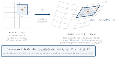
Same mass, different volume

\[ \underbrace{(\psi_{\#}p)\big(\psi(x_0)\big)}_{\text{density at image}} \cdot \underbrace{|\det J_\psi(x_0)|\, h^{d}}_{\text{volume of image}} \;\approx\; \underbrace{p(x_0)}_{\text{density at source}} \cdot \underbrace{h^{d}}_{\text{volume of source}} \]

Every noise point in the cube lands in the image cell, and no other does, because \(\psi\) is a bijection.

The determinant is the exchange rate between volume and density. Where the map expands, the density drops by the same factor.

Divide both sides by the image volume and the theorem falls out. Then say the U2.T2 sentence: there, the same cube is carried along in continuous time and the question becomes how fast its volume grows — the divergence is the volume growth rate, the instantaneous version of this determinant.

Proof sketch, with the gaps named

1. Linear maps move volume by \(|\det A|\): \(\mathrm{vol}(AB) = |\det A|\,\mathrm{vol}(B)\). Gap 1: prove it — factor \(A\) into elementary matrices.
2. A diffeomorphism is locally linear: \(\psi(x) = \psi(x_0) + J_\psi(x_0)(x - x_0) + r(x)\), \(r(x) = o(|x - x_0|)\), so \(\mathrm{vol}(\psi(C_h)) = |\det J_\psi(x_0)|\, h^{d}\,(1 + o(1))\). Gap 2: the \(o(1)\) must be uniform — continuity of the Jacobian.
3. Mass conservation: \(\mathbb{P}[y \in \psi(C_h)] = \mathbb{P}[x \in C_h]\); divide by \(h^{d}\), let \(h \to 0\). Gap 3: this assumes \(y\) has a continuous density. The honest proof shows the substitution rule first, then reads the density off it — dominated convergence.

Waved hands, named as waved hands. Closing them is PS1.3.

Run this live, on the board, in about six minutes. Say “gap” at each gap. The point is not the proof; the point is that the room can see exactly what a complete proof has to add, and that it is first-year analysis, not measure theory.

PS1.3 — your first proof-completion

(a) Linear. \(\mathrm{vol}(AB) = |\det A|\,\mathrm{vol}(B)\) for boxes \(B\), via elementary matrices.

(b) Local. \(\mathrm{vol}(\psi(C_h))/h^{d} \to |\det J_\psi(x_0)|\): sandwich \(\psi(C_h)\) between two scaled copies of the parallelepiped \(J_\psi(x_0)(C_h - x_0)\).

(c) Global. Cut a box into cubes, apply (b), pass to the limit with dominated convergence: \(\int_{\psi(B)} g = \int_B (g \circ \psi)\, |\det J_\psi|\).

(d) Read off the density, both forms, and the log form.

Route fixed on purpose: linearization, not measure-theoretic pushforward machinery. The notes carry the hints.

Assign it here, while the gaps are still on the board and each part visibly closes one. Solutions are comparable because the route is fixed. Due with the rest of PS1.

The fine print

The theorem asks three things of \(\psi\):

1. \(\psi\) is a bijection of \(\mathbb{R}^{d}\) onto \(\mathbb{R}^{d}\);
2. \(\psi\) is differentiable;
3. \(\psi^{-1}\) is differentiable.

Together: a diffeomorphism. Everything built today inherits these hypotheses.

Planted, without comment. Display the three hypotheses, say “diffeomorphism”, and move on. U1.T2 interrogates them. Do not say what the consequences are, and do not draw a picture.

03Compositions and the two costs

Compose invertible maps

\[ \psi^{\theta} = \psi_K \circ \cdots \circ \psi_1 , \qquad (\psi^{\theta})^{-1} = \psi_1^{-1} \circ \cdots \circ \psi_K^{-1} , \qquad \det J_{\psi^{\theta}}(x_0) = \prod_{k} \det J_{\psi_k}(z_{k-1}) \]

Diffeomorphisms compose. The inverse undoes the layers in reverse; the chain rule multiplies the determinants.

Name the intermediate points once: \[ z_0 = x_0, \qquad z_k = \psi_k(z_{k-1}), \qquad z_K = x_1 . \]

A sample flows through the layers. The inverse normalizes data back to the source.

Thirty to forty-two minutes for block C. Say where the two words come from; they are the only etymology of the day.

The log-likelihood telescopes

\[ \log p_\theta(x_1) \;=\; \log p_0(z_0) \;-\; \sum_{k=1}^{K} \log\big|\det J_{\psi_k}(z_{k-1})\big| , \qquad z_K = x_1,\;\; z_{k-1} = \psi_k^{-1}(z_k) . \]

One board line. The chain is computed by running the inverse, from the data point down to the noise point.

Every term must be cheap: for every layer, at every data point, at every training step.

Apply the log form to each layer and add. This is the line that turns a modeling question into a design question, and the next slide is the design question written as a table.

The two costs

Operation	Direction	Needs, per layer	Cost driver
Sampling	forward, \(x_0 \to x_1\)	evaluate \(\psi_k\)	one pass per layer
Density / training	inverse, \(x_1 \to x_0\)	\(\psi_k^{-1}\) and \(\log\lvert\det J_{\psi_k}\rvert\)	the inverse, and the log-det

Versioned: U1.T2 adds a row per architecture; U2.T2 changes what the cells contain; U3.L1 touches neither row.

UP.A §4.4 saw this tension in one dimension, where a monotone map resolves it for free. In \(d\) dimensions the two rows pull against each other. Say that this table is the reading key for the next theory session: every architecture in the zoo is a corner of it.

Why a naive layer is dead on arrival

A dense \(d \times d\) Jacobian: \(O(d^{2})\) to store, \(O(d^{3})\) to take the determinant of — per layer, per data point, per step.

\(32 \times 32\) colour image: \(d = 3072\), so \(d^{3} \approx 3 \times 10^{10}\).

And the inverse of a generic network is not available at all.

The whole architectural zoo of this unit is a list of tricks to make both rows cheap simultaneously.

Say the boxed sentence in those words; it is the unit’s thesis. Blocks D and E give the first two entries in the zoo, and they share one idea.

04NICE: additive coupling

A coupling layer, as a graph

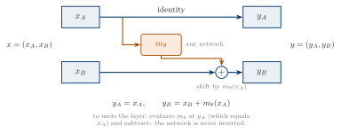
One layer: input \(x\), output \(y\). In the chain of block C, \(x = z_{k-1}\) and \(y = z_k\).

Forty-two to fifty-four minutes for block D. Show the graph before any equation: half the coordinates go straight across, the other half gets shifted by a number computed from the first half. The orange box is the only learned object, and the arrow into it comes from the half that does not move. Say the bridging sentence: inside a layer we write \(x\) and \(y\); in the chain, those are \(z_{k-1}\) and \(z_k\).

Split the coordinates

Partition \(x = (x_A, x_B)\), \(d_A + d_B = d\). Take any network \(m_\theta \colon \mathbb{R}^{d_A} \to \mathbb{R}^{d_B}\):

\[ y_A = x_A , \qquad y_B = x_B + m_\theta(x_A) . \]

Half passes through untouched. The other half is shifted by an amount that depends on the untouched half only (Dinh, Krueger, and Bengio 2015, sec. 3.2).

BOARD 3 starts here, and it stays up through block E, because RealNVP’s Jacobian is obtained by editing this one in place.

The Jacobian, on the board

Order the coordinates \((x_A, x_B)\) and differentiate block by block: \[ J_\psi(x) = \begin{bmatrix} I_{d_A} & 0 \\[4pt] \dfrac{\partial m_\theta}{\partial x_A}(x_A) & I_{d_B} \end{bmatrix} \quad\Longrightarrow\quad \det J_\psi(x) = 1 . \]

Block lower-triangular: the determinant is the product of the diagonal blocks. The expensive block never enters.

Inverse, free: \(\;x_A = y_A , \quad x_B = y_B - m_\theta(y_A) .\)

Derive it on BOARD 3, all four blocks. Circle the lower-left block and say it is the Jacobian of a network, the one expensive thing here, and it does not matter. Then write the inverse under it: one subtraction, one evaluation of the same network.

The trick the whole family rides on

Invertibility of the whole does not require invertibility of the parts.

To undo the layer you evaluate \(m_\theta\) at \(y_A\), which you have, because \(y_A = x_A\). You never invert \(m_\theta\).

So \(m_\theta\) can be as deep, as wide, and as non-invertible as you like. Every coupling architecture in this unit rides on this.

Pause here. This is the conceptual punch of the session, and it is easy to say too fast. Ask the room what the network \(m_\theta\) has to satisfy. The answer is “the right input and output sizes”, and nothing else.

The honest limitation

\(\det J \equiv 1\) means the layer preserves volume. So does any stack of them.

A volume-preserving flow cannot concentrate or spread mass. A real dataset has a different spread from \(\mathcal{N}(0, I_d)\).

NICE’s fix: one final diagonal scaling layer, \(y_i = S_{ii}\,x_i\), with \(\log|\det J_\psi(x)| = \sum_i \log|S_{ii}|\). A global rescaling, once.

The next block makes the rescaling local. That is the whole difference.

Set up RealNVP as the minimal fix: keep everything, let the scale depend on \(x_A\). The notes’ Exercise 2 does the scaling layer’s log-det.

05RealNVP: affine coupling

The same graph, with a scale

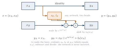
Same untouched half, same conditioner reading it. One new operation on the path of \(x_B\): a scale before the shift.

Fifty-four to seventy-two minutes for block E, the block of the session. Put this graph next to the previous one in the room’s memory: everything is the same except one circle on the lower path. Then write the new \(y_B\) directly under NICE’s on BOARD 3.

Edit one block

Keep the split and the pass-through half. Replace the shift by a shift and a scale, both read off \(x_A\):

\[ y_A = x_A , \qquad y_B = x_B \odot \exp\!\big(s_\theta(x_A)\big) + t_\theta(x_A) . \]

\(s_\theta, t_\theta \colon \mathbb{R}^{d_A} \to \mathbb{R}^{d_B}\) arbitrary networks; \(\odot\) elementwise. The exponential keeps every scale positive (Dinh, Sohl-Dickstein, and Bengio 2017, sec. 3.2).

Write the new \(y_B\) directly under NICE’s on BOARD 3, and keep the graph of the previous slide in view if there is a second screen.

The Jacobian, edited in place

On BOARD 3, edit NICE’s lower-right block in place: erase \(I_{d_B}\), write \(\operatorname{diag}(e^{s_\theta(x_A)})\). The diff is the pedagogy. Then the determinant: product of diagonal blocks, \(1\) times a product of exponentials, and the log turns the product into a sum.

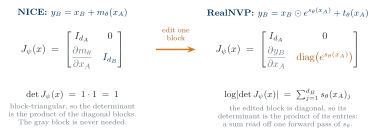
Read off a forward pass

\[ \log\big|\det J_\psi(x)\big| \;=\; \sum_{j=1}^{d_B} s_\theta(x_A)_j \]

A sum read off one forward pass of \(s_\theta\). No \(d \times d\) matrix formed, no determinant computed.

Inverse, closed form: \(\;x_A = y_A, \quad x_B = \big(y_B - t_\theta(y_A)\big) \odot \exp\!\big(-s_\theta(y_A)\big).\)

The sum depends on \(x_A = y_A\) only, so it is available on both sides of the layer — the inverse pass, which training runs, reads it for free.

Subtract, divide. Same cost as the forward pass, same network evaluations. The “both sides” remark is the one U1.L1 uses: during the inverse pass you have \(y_A\), and that is all the sum needs. Exercise 3 in the notes checks the sign.

NICE and RealNVP, side by side

	NICE (additive)	RealNVP (affine)
Layer	\(y_B = x_B + m_\theta(x_A)\)	\(y_B = x_B \odot e^{s_\theta(x_A)} + t_\theta(x_A)\)
\(\log\lvert\det J_\psi\rvert\)	\(0\)	\(\sum_j s_\theta(x_A)_j\)
Inverse	subtract; one pass of \(m_\theta\)	subtract, divide; one pass of \(s_\theta, t_\theta\)
Volume	preserved; a global scaling layer at the end	changed locally, per layer
Untouched half	\(x_A\), read by the conditioner	\(x_A\), read by the conditioner

Both rows of the two-costs table are one conditioner pass per layer, in both directions, for both layers.

The static artifact of the edit-in-place. One minute; the room should be able to reproduce every cell from the board.

What one layer does to a grid

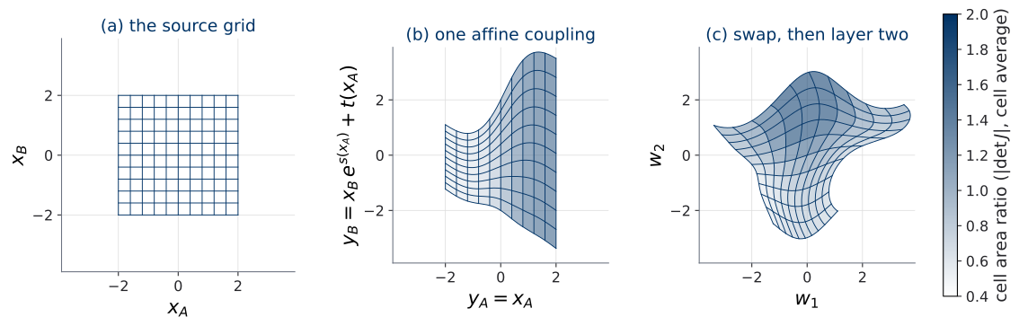
Shading is the cell’s area ratio, \(|\det J|\) averaged over the cell: constant down each column, because it depends on \(x_A\) alone.

Hand-chosen \(s\) and \(t\), not trained — say so. Panel (b): vertical lines stay vertical and in place, horizontal lines bend, the shade is \(e^{s(x_A)}\) and it is the same all the way down a column. The axes are named \(x_A, x_B\) on purpose: \(x_1\) is the data point in this course. Panel (c) is block F in advance: after a swap and a second layer, everything moves. The script checks all three claims numerically before it draws (agreement to \(5 \times 10^{-8}\) or better; the two log-det checks to \(2 \times 10^{-10}\)).

A numerical aside, for the lab

\(e^{s}\) overflows in single precision near \(s \approx 88\). \(e^{-s}\) in the inverse divides by almost zero when \(s\) is large.

Early in training \(s_\theta\) is a random network, and both happen.

Implementations bound the scale: \(s = c \cdot \tanh(\tilde s)\) before the exponential.

One slide. The lab (U1.L1) shows the loss curve when you forget.

No dwelling. This exists so the lab’s failure mode has a name when it appears.

The training loss, in full

\[ \begin{aligned} \mathcal{L}(\theta) &= -\;\mathbb{E}_{x_1 \sim q}\Big[ \log p_0(z_0) - \sum_{k=1}^{K} \log\big|\det J_{\psi_k}(z_{k-1})\big| \Big] , \\[4pt] &\phantom{=} z_K = x_1,\qquad z_{k-1} = \psi_k^{-1}(z_k) . \end{aligned} \]

The subscript on \(\mathbb{E}\) is mandatory, and this is the first loss of the course where it is enforced. Each log-det is a sum of scales at the untouched half of \(z_{k-1}\).

PS1.4 is exactly the bookkeeping of this expression for a three-layer RealNVP. Assigned now.

Notation discipline moment. Write the loss on the board with the subscript, point at it, and say the primer’s rule: every expectation in every loss carries its sampling subscripts. Then assign PS1.4 while the expression is up.

PS1.4 — the bookkeeping

\(\psi^{\theta} = \psi_3 \circ \psi_2 \circ \psi_1\); coordinates of a vector written \((\xi_1, \dots, \xi_4)\) (\(x_1\) stays the data point). Layers 1 and 3 condition on \((\xi_1, \xi_2)\) and move \((\xi_3, \xi_4)\); layer 2 the reverse.

(a) Write the inverse pass: \(z_2, z_1, z_0\) from a data point, in the order computed.

(b) Write \(\log p_\theta(x_1)\) fully explicitly: every log-det as its sum of scales, every scale at the correct intermediate point.

(c) Write the minibatch loss, sample mean in place of the expectation, subscript kept.

(d) Replace \(\psi_2\) by a swap of the halves. Redo (b). Which term changes?

Mechanical on purpose: the notation of the loss through your hands once, before U1.L1 puts it through code.

Two minutes. Part (d) is the permutation check of block F, done in symbols.

06Masks, partitions, permutations

\(x_A\) is never touched, so alternate

A coupling layer leaves \(x_A\) exactly as it found it. Same split forever means a model of \(x_B\) only.

• Alternate the split: layer \(k\) moves \(B\), layer \(k+1\) moves \(A\). Two layers move everything; three let everything influence everything.
• Permute between layers: a fixed \(P\) between couplings. Bijection, inverse \(P^{\top}\), \(|\det P| = 1\), so its log-det is zero.

Check the permutation in your head now; check it in code next session (U1.L1).

For images: binary masks, checkerboard and channel-wise. One line; that is U1.L2.

Seventy-two to eighty-two minutes for block F. The “three layers” remark is NICE’s own observation (§3.2). The mask line is one sentence and a pointer.

Depth as the lever

With alternation in place, a stack of \(K\) affine coupling layers moves every coordinate, and the composed Jacobian is dense once \(K \ge 3\).

The natural next belief: with enough layers, a coupling flow reaches anything. Asserted today. Not proven.

How expressive is a stack of these, really?

Written on the board next to the session question. Answered in U1.T2.

BOARD 1: write the depth question next to the session question. This is the calibrated teaser. Do NOT preview the answer, and do not draw any picture of what a flow cannot do. The fine print of block B comes back with it.

07Training loop and close

The training loop, in full

for x1 in loader:                    # minibatch, x1 ~ q
    loss = -flow_log_prob(x1).mean()  # minus mean log p
    opt.zero_grad()
    loss.backward()
    opt.step(); sched.step()

flow_log_prob is the telescoped log-likelihood: inverse chain, plus \(\log p_0(z_0)\), minus the \(K\) sums of scales. You write it in U1.L1. opt: AdamW, LR \(3 \times 10^{-4}\), weight decay \(0.01\); sched: warmup, then cosine.

Bootcamp readers: training-loop-template with a new loss line, under optimizer-schedule-defaults. For everyone else, the box is the whole definition.

Eighty-two to ninety minutes for block G. The parity rule in action: the loop is on the slide in full, so PESC reads a definition and PGMAT reads a callback. Do not explain AdamW or the schedule; the defaults are named and that is all today needs.

Reading the board

On the board	Status
The session question — what must \(\psi^{\theta}\) satisfy?	Answered: a diffeomorphism, built from layers whose inverse and log-det are cheap.
The depth question — how expressive is a stack?	Open. U1.T2.
The fine print — bijection, differentiable, both ways	Unexamined. U1.T2.

Read BOARD 1 out loud, both questions. Answer the first in one line. Leave the second. Point at the three hypotheses and say they have not been examined.

What comes next

• Next session (U1.L1): build it. An affine coupling layer and a permutation from scratch, the sum of scales checked against an autodiff Jacobian, trained on 2D toy data by the loop you just saw.
• The theory session after (U1.T2): the rest of the zoo, and where its expressivity claims break.

Assigned today: PS1.3 (the proof) and PS1.4 (the bookkeeping).

Two sentences and out. The notes’ §8 has four exercises with answers for anyone who wants the permutation and scaling-layer checks written out.

References

Dinh, Laurent, David Krueger, and Yoshua Bengio. 2015. “NICE: Non-Linear Independent Components Estimation.” In International Conference on Learning Representations, Workshop Track. https://arxiv.org/abs/1410.8516.

Dinh, Laurent, Jascha Sohl-Dickstein, and Samy Bengio. 2017. “Density Estimation Using Real NVP.” In International Conference on Learning Representations. https://arxiv.org/abs/1605.08803.

Papamakarios, George, Eric Nalisnick, Danilo Jimenez Rezende, Shakir Mohamed, and Balaji Lakshminarayanan. 2021. “Normalizing Flows for Probabilistic Modeling and Inference.” Journal of Machine Learning Research 22 (57): 1–64. https://arxiv.org/abs/1912.02762.