U0.T4 — Architectures for the Road and Evaluation

Flow-Based Generative Models · UFRJ · 2026.2

01The parts list

One signature, for the rest of the course

Every network we train from here on has the same shape:

\[ f_\theta \colon \; \underbrace{(B, C, H, W)}_{x} \; \times \; \underbrace{(B,)}_{t} \; \longrightarrow \; (B, C, H, W) \]

In U3 this object is the learned velocity field \(u_t^\theta(x)\). Today it is just “the network”.

Two questions, and the session is their answer: what goes inside, and how does \(t\) get in?

Write the signature on the board now and do not erase it for the whole session. Every block points back at it. If a student asks what B, C, H, W are: batch, channels, height, width — the shape of a batch of images.

The code contract, stated once

t is a (B,) tensor of floats in \([0,1]\). \(t=0\) is noise, \(t=1\) is data.

Not an integer index. Not a step count. Code needing another time variable converts outside the network.

The diffusion literature counts time backwards, in discrete steps. The moment a network accepts an integer timestep, that convention is in the codebase — and every later translation becomes a silent sign error.

This line is asserted inside unet-skeleton in the next lab session. Say that now: the contract is enforced by code, not by goodwill.

And how do we know a model is any good?

Three answers, all in the evaluation block at the end:

1. Likelihood — what it measures, and why a great score is compatible with terrible samples.
2. FID — the field’s standard, and the three caveats that are part of its definition.
3. Precision and recall — the two different ways a model can be bad, separated.

Question of the day: what are the parts, and what is the ruler?

02Attention in one pass

The need

A convolution mixes a pixel with its neighbours. Its reach grows only by stacking layers.

Sometimes a position needs information from a distant position — and which position depends on the content, not on the geometry.

Attention is the mechanism that lets a position ask for what it needs.

This is the only session in the course that teaches attention. After today it is vocabulary. Say that out loud so nobody waits for a second pass.

Queries, keys, values

Each of \(n\) positions produces three vectors, by linear maps of its own representation:

• query \(q_i \in \mathbb{R}^{d_k}\) — what this position is looking for;
• key \(k_j \in \mathbb{R}^{d_k}\) — what position \(j\) advertises;
• value \(v_j \in \mathbb{R}^{d_v}\) — what position \(j\) hands over.

Stack them as the rows of \(Q\), \(K\), \(V\).

The operation

\[ \operatorname{Attn}(Q, K, V) = \operatorname{softmax}\!\left( \frac{Q K^{\top}}{\sqrt{d_k}} \right) V \] Rows of \(A = \operatorname{softmax}(QK^\top/\sqrt{d_k})\) are non-negative and sum to one.

Why \(\sqrt{d_k}\)? With unit-variance entries, \(q \cdot k\) has variance \(d_k\). Unscaled, the scores grow with the width, the softmax saturates, and the gradient dies.

Same variance-propagation argument as U0.T2’s initialization rule.

If they have seen attention before, the sqrt(d_k) argument is usually the part they cannot reproduce. Spend the thirty seconds.

Three positions, done by hand

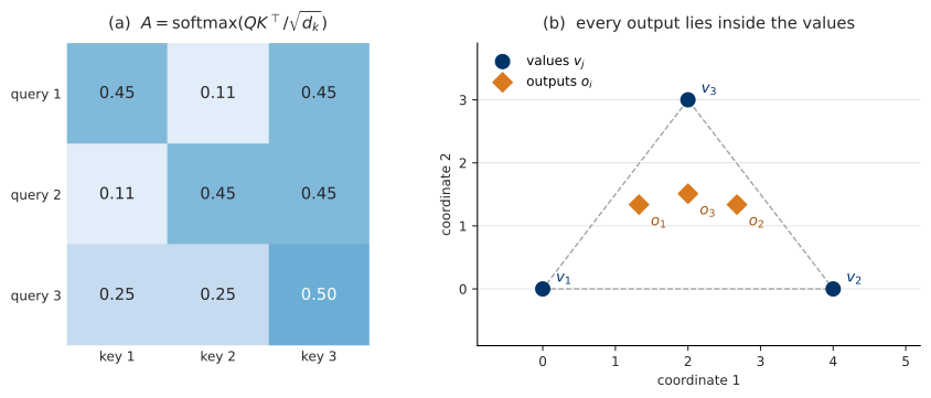
Every output is a convex combination of the value vectors. Attention cannot invent content — only redistribute it.

Q, K, V for this figure are small integers, printed in the notes. Invite anyone to check row 3 by hand: 0.25, 0.25, 0.50.

The same thing, turning

Every number here is computed by the same code as the static figure — the attention rows, the swept locus, the peak weight. Two things to point at. (1) The row is a probability vector, so it IS the barycentric coordinate of the output: watching the orange point fail to escape the triangle and reading “the rows sum to one” are the same fact. (2) The ending is the softmax doing its job: lengthen the query, the scores grow, the row goes one-hot, and the output lands on a value. Even there it is inside. Let it run; it is deliberately slow.

Multi-head, in one slide

One attention operation expresses one notion of relevance. Run \(h\) of them in parallel, on projections into lower-dimensional subspaces:

\[ \begin{aligned} \operatorname{head}_m &= \operatorname{Attn}(X W^Q_m, X W^K_m, X W^V_m) \\ \operatorname{MHA}(X) &= [\operatorname{head}_1, \dots, \operatorname{head}_h] \, W^O \end{aligned} \]

Each head can specialize. The cost is unchanged: per-head width is the full width divided by \(h\).

Attention does not know where anything is

For any permutation matrix \(P\): \[ \operatorname{Attn}(PQ, PK, PV) = P \operatorname{Attn}(Q, K, V) \]

Permute the positions, and the outputs permute. Nothing else changes.

Consequence: anything the network must know — position, time — has to be injected into the representation. That is the conditioning block.

The figure script checks this numerically and the error is exactly 0.0. This slide is the hinge into the conditioning block: hold the thought.

The cost decides the architecture

\(QK^\top\) has \(n^2\) entries: \(O(n^2 d_k)\) time, \(O(n^2)\) memory.

For an image as a sequence of pixels, \(n = HW\):

Image	\(n\)	entries per head
\(32 \times 32\)	\(1\,024\)	\(\approx 10^6\)
\(256 \times 256\)	\(65\,536\)	\(\approx 4 \times 10^9\)

So: attention only where the resolution is low. Or first reduce \(n\) — the transformer route.

Where you will meet this again

The U6 seminar papers are transformer-native and assume all of the above without a word.

The architecture in the preview block is nothing but this block, repeated.

Today is the only time attention is taught. After this, it is vocabulary.

03U-Net anatomy

The shape problem

The signature asks for \((B,C,H,W) \to (B,C,H,W)\). That is demanding:

• the output needs detail — it is per-pixel, and blurred is wrong;
• each pixel’s decision needs global context — a \(3\times3\) neighbourhood cannot tell a 3 from an 8.

Full resolution throughout: has the detail, needs impractical depth for the context (U0.T2’s receptive-field computation).

Downsample: gets the context, destroys the detail.

Do both, then reconnect

This is the named asset slide-unet-anatomy. It is the build map for the next lab session, so walk every box: encoder path, bottleneck with attention, decoder path, skips, and the orange conditioning bus we unpack in the next block.

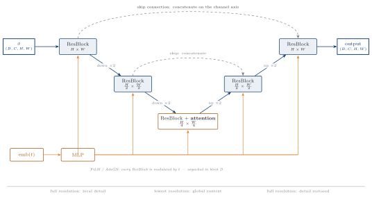
The three parts, and the dashed arcs

• Encoder — ResBlocks and downsampling; resolution halves, channels grow.
• Bottleneck — lowest resolution, so every unit sees the whole image, and attention is finally affordable.
• Decoder — mirrors the encoder, upsampling back.

Skip connections concatenate on the channel axis. Not addition: the decoder receives the encoder’s features as extra channels and learns what to do with them.

Concatenation vs addition is a real question a student will ask. Addition assumes the two representations are commensurate. Concatenation makes no such assumption and costs channels.

Why the skips are not optional

The bottleneck representation is small by construction.

Detail that is needed to reconstruct a pixel, and is not predictable from context, cannot pass through it — not because training failed, but because there are fewer numbers than the detail requires.

The skips route that detail around the bottleneck.

So a U-Net is both ideas from U0.T2 at once: multiscale, and residual.

The block interior is the recipe card

Nothing new inside a ResBlock — U0.T2’s defaults, unchanged:

• GroupNorm, not BatchNorm. A generative model is evaluated one sample at a time; batch statistics would make the output depend on what else was in the batch.
• SiLU activation.
• Zero-init the last convolution, so the block starts as the identity.

This architecture, plus the conditioning of the next block, is unet-skeleton — built in the next lab session, trained for the rest of the course.

04Time conditioning

The requirement

We do not train one network per time.

One network, all \(t \in [0,1]\). So \(t\) is an input: one continuous scalar per example, which must influence every layer at every resolution.

Two decisions:

1. how to turn one number into something usable;
2. how to deliver it everywhere.

This is the block to slow down on. Per the pre-plan it is emphasized, because every later model in the course is time-conditioned. Board 2 goes up here.

Why not just feed \(t\)?

A single input coordinate enters the first layer through a single column of weights.

To make its effect on the computation detailed, every downstream layer must reconstruct that dependence from one nearly-linear signal.

The network can do it. It wastes capacity doing it.

Remedy: expand \(t\) over a geometric ladder of frequencies, so coarse and fine differences in \(t\) are directly available as separate coordinates.

The ladder — the course spec

For t a (B,) float tensor in \([0,1]\), width \(d_{\text{emb}}\), \(\mathrm{half} = d_{\text{emb}}/2\): \[ \begin{aligned} \omega_k &= (10^4)^{-k/\mathrm{half}}, \quad k = 0, \dots, \mathrm{half}-1 \\ \mathrm{emb}(t) &= \big[\sin(\omega_k \cdot 1000\,t) \,;\, \cos(\omega_k \cdot 1000\,t)\big]_k \end{aligned} \]

The factor \(1000\) is the only rescale. Reference implementations were calibrated to a thousand-step schedule; matching them means a library cross-check catches real bugs, not conventions.

Outside this line, \(t\) is a float in \([0,1]\). The FM arrow is untouched.

What the ladder actually does

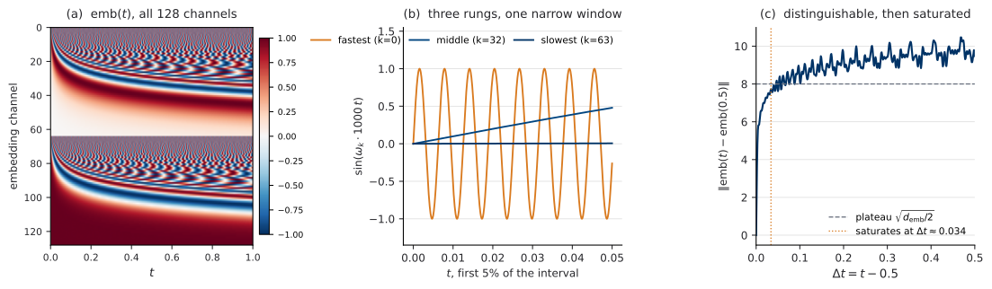
Slowest rung: monotone over the whole interval — “early or late?”. Fastest: \(\approx 159\) cycles — resolves \(\Delta t \sim 10^{-3}\).

The right panel is the honest limit and is worth stating: distance saturates at about delta-t = 0.034. The embedding is not a global ruler for time; it separates nearby times sharply and calls far-apart times simply different.

The ladder, as hands on dials

Each rung is a hand turning at its own rate: blue at t = 0.5, orange at t’. The distance curve on the right is not an analogy — it is exactly the sum of the phase differences on the left, and the precompute asserts that identity. Point at the first beat: the fast hand has gone round eight times while the slow hand has barely stirred, which is what “several resolutions at once” means. Then let the honest ending land: the curve plateaus at about Δt = 0.034 and never rises again. The embedding is a fine ruler nearby and no ruler at all far away. Do not skip this — it is the caveat students would otherwise carry away wrong.

Getting it into every block

Concatenating the embedding is possible and wasteful. Modulate instead:

With \(\hat h\) the output of the block’s normalization layer: \[ h \leftarrow \big(1 + \gamma(t)\big) \odot \hat h + \beta(t) \] \(\gamma(t), \beta(t) \in \mathbb{R}^{C}\): one pair per channel, from a small MLP on \(\mathrm{emb}(t)\).

AdaGN is this, with GroupNorm as the normalization. Same operation, different name.

Three things about that equation

• Written \(1 + \gamma\), so \(\gamma = 0\) means no modulation. With a zero-initialized projection, the block starts out ignoring \(t\) and learns to use it.
• Cheap: two numbers per channel per block, against thousands in a conv kernel.
• Applied after the normalization — which is the whole point. Normalization has just removed the scale and offset; modulation puts a \(t\)-dependent one back.

In the block

Board 2: draw this equation next to a ResBlock sketch as it appears. The chain around it is the U0.T2 recipe card, unchanged — only the orange box is new today.

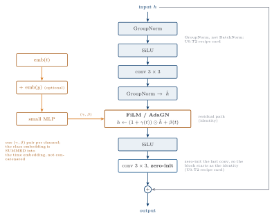
One more signal, for free

The model should also depend on a class label \(y\)? Embed \(y\) to the same width and add:

\[ c = \mathrm{emb}(t) + \mathrm{emb}(y) \]

Feed \(c\) through the same projection, to the same \((\gamma, \beta)\). Nothing else changes.

Summing keeps the width fixed, so the modulation path does not grow with the number of signals.

A class-conditional model built this way returns in U3.

One sentence and move on. No null token, no dropout, no guidance — that is U3.L3’s material and importing it here would spoil it.

The artifact

1. Ladder — \(\omega_k = (10^4)^{-k/\mathrm{half}}\), argument \(\omega_k \cdot 1000\,t\), sine and cosine concatenated.
2. Projection — small MLP \(\to (\gamma, \beta)\) per block, per channel; zero-initialized.
3. Application — after the normalization, in every ResBlock at every resolution.
4. Extra conditioning — embedded to the same width and summed, never concatenated.

Cited by the next lab session, by every U3 lab, and by U5.T1.

Where you will meet this again

Every velocity field, every score network, every diffusion model you will read in this course uses exactly this block.

It is the single most transferable slide of the bootcamp.

05A preview: the transformer backbone

Patchify, then it is just a transformer

Replace the U-Net entirely. Cut the input into \(p \times p\) patches, embed each linearly into a token, add sine–cosine positions:

\[ T = (I/p)^2 \ \text{tokens of width } d \]

Halving \(p\) quadruples \(T\) — and by the cost slide, at least quadruples the compute.

From there: a stack of standard transformer blocks.

adaLN-zero — the same idea, one layer over

Point at the symmetry with the conditioning block explicitly: scale and shift regressed from the SUM of the t and class embeddings, applied at LayerNorm instead of GroupNorm. The alpha gate is the new part, and its zero-init is the recipe card’s law again.

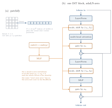
Why the zero matters

The \(\alpha\) gate sits immediately before each residual connection, and its projection is initialized to zero.

So at initialization every block is exactly the identity, and the network starts as a pass-through.

Reported effect: adaLN-zero reaches roughly half the FID of in-context conditioning at 400k iterations, at negligible extra cost (Peebles and Xie 2023).

How the conditioning enters changes model quality substantially.

One sentence on scale, then stop

Across model sizes from 12 to 28 layers, and across patch sizes, larger transformer backbones give better samples — consistently, without special handling.

Why, and at what cost: U5.T1. Preview only.

06Evaluating generative models

We can build them. What is the ruler?

Three candidates, and the section is organized around what each one misses:

1. Likelihood — measures coverage; says surprisingly little about samples.
2. FID — the field’s standard; three caveats that are part of its definition.
3. Precision / recall — separates the two ways a model can be bad.

No single number does the job. That is not a gap in the course; it is the state of the field.

Bits per dimension

\[ \mathrm{BPD}(\theta) = -\frac{1}{d \log 2} \; \mathbb{E}_{x \sim q}\big[\log p_\theta(x)\big] \] Lower is better. It is a compression rate: bits per dimension to encode a test example under a code built from \(p_\theta\).

BPD measures coverage. Assign low density where the data lives and \(-\log p_\theta(x)\) punishes you without limit.

That is a real virtue — and it is why likelihood is still the right score for density estimation.

Great likelihood, terrible samples

Take a model that samples from a good generator with probability \(1-\varepsilon\), and from pure noise with probability \(\varepsilon\).

Its log-likelihood is within \(\log\frac{1}{1-\varepsilon}\) of the good model’s. Divided by \(d\), that is invisible for image-sized \(d\).

Its samples are garbage a fraction \(\varepsilon\) of the time.

The damage hides in directions the average does not weight (Theis, Oord, and Bethge 2016).

This is the single most useful thing in the likelihood part. If the block runs long, cut the taxonomy re-show, not this.

And sometimes there is no number at all

Re-show the taxonomy from U0.T3 — now read it as an evaluation table:

Family	Exact likelihood?	Then evaluate with
Autoregressive	yes	BPD, and samples
Normalizing flows	yes	BPD, and samples
VAE	bound only (ELBO)	ELBO, FID, panels
GAN	no density at all	FID, precision / recall

Any protocol that requires likelihood cannot compare across the columns.

FID: the recipe

1. Push real and generated samples through a fixed feature extractor.
2. Fit a Gaussian to each feature set.
3. Report the Fréchet distance between the two Gaussians.

\[ \begin{aligned} \mathrm{FID} =\;& \lVert \mu_r - \mu_g \rVert^2 \\ &+ \operatorname{Tr}\!\left(\Sigma_r + \Sigma_g - 2(\Sigma_r \Sigma_g)^{1/2}\right) \end{aligned} \] The Gaussian fit is an assumption: only the first two moments are compared.

The three caveats are part of the definition

1. Comparable only at identical extractor, preprocessing and sample count. An FID is a property of a model and a protocol.

2. Biased upward; the bias falls like \(1/n\). The FID of a set against its own distribution is not zero.

3. The extractor decides what “similar” means. Inception features are ImageNet-shaped. This course pins a small MNIST classifier for MNIST, and reserves Inception for CIFAR and beyond.

Measured, on a case with a known answer

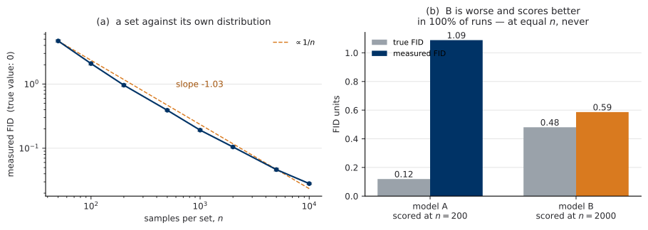
Left: both sets from one distribution, true FID \(= 0\). Measured \(4.7\) at \(n=50\); \(0.028\) at \(n=10^4\); slope \(-1.03\).

Everything plotted on the left panel is bias, because the true value is exactly zero by construction. That is why the toy is a Gaussian: we know the answer.

The consequence, and it is a rule

Two models: true FID \(0.12\) and \(0.48\). B is worse, by a gap of \(0.36\).

• Score A at \(n=200\), B at \(n=2000\): B wins in 40 of 40 trials (\(0.59\) against \(1.09\)).
• Score both at the same \(n\): the ranking is correct in every trial.

The bias is systematic, so at equal \(n\) it lands on both and cancels.

The ranking inverts exactly when the difference in bias exceeds the true gap. (\(200\) vs \(2000\): difference \(0.86 > 0.36\), always inverts. \(500\) vs \(5000\): \(0.34 < 0.36\), inverts \(17.5\%\) of the time.)

Watch the ranking break

The grey base of each bar is the true FID; the coloured top is the bias. Beat two is the one that matters most and is easiest to skip: at equal n the same bias lands on both bars and the ranking SURVIVES — measured, zero inversions in forty runs. Only then does B get more samples, and the bars cross exactly where the bias difference passes the true gap, at n = 400. That is why the harness logs extractor, preprocessing and sample count beside every FID: not as bookkeeping, but because without them the number cannot be compared to anything.

Precision and recall

FID is one number. A model can be bad in two different ways.

Approximate each set’s support by a union of balls — around each point, out to its \(k\)-th nearest neighbour in that set. Then:

• precision = fraction of generated points inside the real support → fidelity;
• recall = fraction of real points inside the generated support → coverage.

The taxonomy gets its diagnosis language

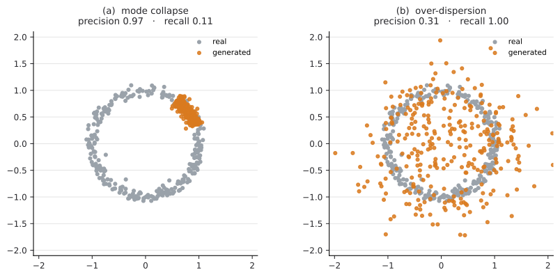
Mode collapse (GANs): high precision, low recall. Over-dispersion: the reverse.

The numbers under the panels are measured with the real k-NN estimator, not chosen for the slide. Likelihood-trained models sit at the right-hand end: BPD punishes missing mass and tolerates spurious mass. That is the honest version of “VAE samples are blurry”.

Where you will meet this again

U3.L2 measures the number of function evaluations against FID.

U3.L3 sweeps a conditioning strength against FID — where the fidelity-versus-coverage trade becomes something you watch move.

The harness you build in the next lab session is the instrument.

Precision and recall stay concept-only: vocabulary for reading papers, not code in the harness.

07Close

The next lab session builds two things

1. The time-conditioned U-Net — the anatomy slide assembled, conditioning wired into every block. Interface frozen that session:

forward(x, t, y=None)   # t: (B,) float in [0, 1]

2. The evaluation harness — FID and BPD implemented, the caveats enforced by code. Calibrated before it is trusted, then pointed at your U0.L3 VAE.

Both are PS0 components.

PS0 assembly, two more pieces lit up

Piece	From	Status
training-loop-template	U0.L1	built
hygiene-stack	U0.L2	built
vae-mnist-scratch	U0.L3	built
unet-skeleton	U0.L4	next session
eval-harness	U0.L4	next session

Exit line: you now know what the parts are, and what the ruler is. Next session you build both.

Re-show the PS0 assembly slide from U0.L3 if it is still to hand; this table is its continuation. Close on the exit line.

References

Peebles, William, and Saining Xie. 2023. “Scalable Diffusion Models with Transformers.” In IEEE/CVF International Conference on Computer Vision. https://arxiv.org/abs/2212.09748.

Theis, Lucas, Aäron van den Oord, and Matthias Bethge. 2016. “A Note on the Evaluation of Generative Models.” In International Conference on Learning Representations. https://arxiv.org/abs/1511.01844.