U1.L2 — Multi-Scale Flows on Images

Flow-Based Generative Models · UFRJ · 2026.2

01Why images change the problem

Where this session sits

Session	What happened
U1.L1	a coupling flow from nothing, trained on points in the plane
U1.T2	the zoo: Glow’s layers, MAF/IAF, what a flow cannot represent
U1.L2 — today	the same algebra on images: integers, \(d = 784\), one frozen protocol
U2.T1	depth becomes continuous

This session is elastic: the first one cut if the calendar slips. The notebook and the notes are written to be read without a lecturer.

Zero to eight minutes for block A. Say the joint-audience sentence once: this lab depends on U1.T2 and U1.L1 and on nothing else; four modules arrive as given code, and their contracts are on the slide after next. Notebook open on the projector from here on. Board 1 is written during block B and stays up through block E.

Three things you leave with

1. bpd-protocol — observation model, dequantization, preprocessing, evaluation, frozen with constants. A likelihood number without it is not a result.
2. The multi-scale bookkeeping, executable — squeeze: log-det exactly \(0\); factor-out: a partition, not a transform; a table whose rows add up to log_prob.
3. A course-internal comparison under one protocol — and the list of reasons a number copied from a paper is not on the same axis.

Not on the list: a metric for samples. That is U3.L2.

Two problems with naive reuse of U1.L1

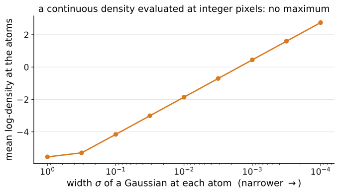
The observations are atoms. A pixel is \(k \in \{0, \dots, 255\}\); 81% of MNIST test pixels are exactly \(0\). A continuous density at an integer is not a mass, and maximizing it on atoms has no maximum:

The dimension is \(784\). A U1.L1 conditioner at \(d = 784\), width \(512\): \(0.9\) M parameters per coupling layer.

The figure is computed, not sketched: one pixel, 256 Gaussians at the atoms, scored at the atoms; the mean log-density climbs by 8.3 nats as the width goes from 1 to 1e-4. Neither problem is the change-of-variables theorem. Block B fixes the first, block C organizes the second.

Given code, four modules

Module	Built in	Used today
common/train.py	U0.L1–L2	set_seed, Trainer.fit, as in U1.L1
common/eval.py	U0.L4	bpd only: the continuous-density term; signature in block B
common/coupling.py	U1.L1	the affine algebra; nothing new
common/multiscale_flow.py	today	Logit, Squeeze2d, ImageAffineCoupling, MultiscaleFlow

The bootcamp is provenance, not a prerequisite: each contract is on the page that uses it.

The data-loader rule

Load MNIST as stored: uint8, values in \(\{0, \dots, 255\}\). Keep it that way until the dequantization cell.

ds = datasets.MNIST(str(DATA), train=False,
                    download=False)
k_test = ds.data.clone().unsqueeze(1)  # uint8 (N,1,28,28)

Keep ToTensor() out: it divides by 255, not \(256\), and hides the factor whose logarithm becomes the \(+8\).

Checkpoint 0: dtype, range, and what ToTensor() would have done.

The observation model, in one figure

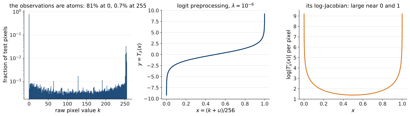
Left: atoms. Middle: the logit layer of block B. Right: its per-pixel log-Jacobian — large exactly where the pixels are.

02Dequantization and bits per dimension

Uniform dequantization

For raw \(k \in \{0,\dots,255\}^D\) and \(u \sim \mathrm{Unif}([0,1)^D)\):

\[ x = \frac{k + u}{256} \in [0,1)^D \]

The discrete model a continuous density \(p_X\) induces is the mass of the cell: \[ P_\theta(k) = \int_{[k/256,\,(k+1)/256)} p_X(x)\,dx = \frac{1}{256^{D}}\;\mathbb{E}_{u \sim \mathrm{Unif}([0,1)^D)}\!\left[p_X\!\left(\tfrac{k+u}{256}\right)\right]. \]

Board 1 starts here: write x = (k+u)/256, the cell, the substitution with the constant Jacobian 256^{-D}. Then the next slide’s inequality goes under it, and stays.

The bound, and its direction

\[ \begin{aligned} \log P_\theta(k) &= \log \mathbb{E}_{u}\!\left[p_X\!\left(\tfrac{k+u}{256}\right)\right] - D\log 256 \\ &\ge \mathbb{E}_{u \sim \mathrm{Unif}([0,1)^D)}\!\left[\log p_X\!\left(\tfrac{k+u}{256}\right)\right] - D\log 256 \end{aligned} \]

Jensen; \(\log\) is concave.

What a flow trains on and reports is the right-hand side: a lower bound on discrete log-mass — an upper bound on discrete NLL, in expectation over \(u\) (Theis, Oord, and Bethge 2016, sec. 3.1).

Training on \(x\) pushes up a lower bound on the discrete likelihood. That is why it is legitimate.

A one-sample estimate is not an exact bound

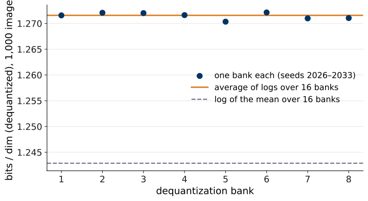
Eight one-sample banks on \(1{,}000\) images: spread 0.0018 bits/dim around the sixteen-bank average 1.272. Dashed, 1.243: the log-of-mean over sixteen banks — a tighter lower bound, still in expectation.

The sentence to say: a finite Monte Carlo estimate of the expectation fluctuates around the bound value. Do not call one draw an exact bound. Several draws per image and variational dequantization are named, not done.

Logit preprocessing is a flow layer

\[ \begin{aligned} a &= \lambda + (1-2\lambda)\,x, \qquad \lambda = 10^{-6}, \\ y &= T_\lambda(x) = \log a - \log(1-a), \end{aligned} \] \[ \log\lvert\det J_{T_\lambda}(x)\rvert = \sum_{j=1}^{D}\Big[\log(1-2\lambda) - \log a_j - \log(1-a_j)\Big] \]

\[ \log p_X(x) = \log p_Y\big(T_\lambda(x)\big) + \log\lvert\det J_{T_\lambda}(x)\rvert \]

TODO 1.2 — the Jacobian by hand

Logit.inverse(x) is the density direction \(x \to y\) (course contract: forward is \(\psi\), so the logit is an inverse). It returns the Jacobian as its second output.

def logit_logdet(x, lam=LAM):
    a = lam + (1 - 2 * lam) * x
    return (math.log(1 - 2 * lam) - torch.log(a)
            - torch.log1p(-a)).flatten(1).sum(1)

Checkpoint 1.2: your sum against the layer’s, float64; about 4620 nats per image on test data. The preprocessing term is never hidden or dropped.

Bits per dimension, and the \(+8\)

The harness contract, frozen in U0.L4 — the continuous-density term only:

bpd(log_prob_nats_per_example, num_dims)
    = -mean(log_prob_nats_per_example)
      / (num_dims * log(2))

\[ \widehat{\mathrm{bpd}}_{\mathrm{deq}} = \mathrm{bpd}_{\mathrm{cont}} + 8, \qquad \frac{\log 256}{\log 2} = 8 \]

Two anchors: a uniform density on \([0,1)^{784}\) reports exactly \(8\) — the raw code. A model that concentrates has \(\mathrm{bpd}_{\mathrm{cont}} < 0\): the reference reports \(-6.700 + 8 = 1.300\).

Board 1, second half: -D log 256 divided by D log 2 is -8 in the log-mass, so +8 in the bits. Say where it lives: in the protocol, not in the harness.

Artifact bpd-protocol — frozen

• raw 8-bit test split; \(D = 784\); full \(N = 10{,}000\) unless a subset is labelled
• one fixed dequantization bank per image: K_deq = 1, seed \(2026\), CPU, test order
• \(\lambda = 10^{-6}\); the logit Jacobian included before eval_harness.bpd
• reported: eval_harness.bpd(log_prob_x, 784) + 8
• every report logs: dataset/split, \(N\), seed and K_deq, \(\lambda\), checkpoint hash and config

The bank’s SHA-256 is recorded and asserted. Multi-sample and variational dequantization: named, outside this lab.

TODO 1.3 — the protocol, and the arithmetic beside it

def bpd_protocol(log_prob_x):
    return bpd(log_prob_x, D) + 8.0

def bpd_manual(log_prob_x):
    lp = np.asarray(log_prob_x, dtype=np.float64)
    return (-lp.mean() / (D * math.log(2.0))
            + math.log(256.0) / math.log(2.0))

Checkpoint 1.3: agree to \(10^{-12}\); the uniform density reports exactly \(8\); a density of \(e^{784}\) everywhere reports \(8 - 1/\log 2\).

03The multi-scale shell

Three pieces, one contract

# every layer: forward(z) -> (x, logdet_fwd)   psi
#              inverse(x) -> (z, logdet_inv)   psi^-1
Squeeze2d(factor=2)           # inverse SQUEEZES; logdet 0
ImageAffineCoupling(C, mask)  # U1.L1 layer, CHANNEL mask
MultiscaleFlow(shape, levels, # squeeze -> steps -> factor
               steps, hidden) #   out half, per level
  .log_prob(y)   .sample(n, tau)   .bookkeeping(y)

Names follow the density direction, as the papers draw it. The coupling layer is U1.L1’s with a conv conditioner (\(3{\times}3 \to 1{\times}1 \to 3{\times}3\), small nonzero head) and the same tanh bound.

The picture from U1.T2, now code

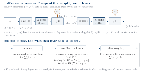
Density direction left to right; sampling runs every arrow backwards. Today the top row becomes code.

Board 2 — squeeze is a permutation, factor-out is a partition

Board 2 is this figure, drawn by hand: the 4x4 with its four fills, the four channels, “log det = 0” beside the squeeze, “a partition, not a transform” beside the factor-out. It stays up for block C.

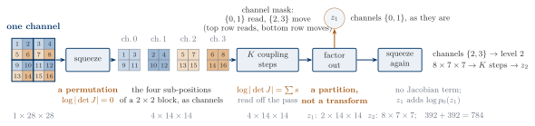
Squeeze: exactly zero

\(1 \times 28 \times 28 \to 4 \times 14 \times 14\): the four entries of every \(2 \times 2\) block become four channels at one position. Nothing is scaled: a permutation of the \(784\) coordinates, \(\log\lvert\det J\rvert = 0\).

A channel mask is a spatial mask. Channel \(0\) holds the top-left of every block, channel \(1\) the top-right, \(2\) and \(3\) the bottom row. Reading \(\{0,1\}\) = reading the top row of every block.

RealNVP alternates spatial checkerboard masks before a squeeze with channel masks after (Dinh, Sohl-Dickstein, and Bengio 2017, sec. 3.6); the course shell uses channel masks only, alternated across steps.

Factor-out: a partition, and the total

\[ \begin{gathered} \log p_Y(y) = \sum_{l=1}^{L} \log p_0(z_l) + \sum_{\text{couplings}} \log\lvert\det J_{\psi_k^{-1}}\rvert, \\ \sum_l \dim z_l = 784 \end{gathered} \]

At the end of a level, channels \(\{0,1\}\) go to \(z_1\) as they are; \(\{2,3\}\) continue at half resolution. No Jacobian term. \(z_1\) contributes \(\log p_0(z_1)\) at the end (Dinh, Sohl-Dickstein, and Bengio 2017, eqs. 13–16).

Reference model: \(z_1\) is \(2 \times 14 \times 14\) (\(392\)), \(z_2\) is \(8 \times 7 \times 7\) (\(392\)).

TODO 2.1 — squeeze, checked

sq = Squeeze2d(2)
z, ld = sq.inverse(y8)            # (8, 4, 14, 14)
y_back, ld_back = sq.forward(z)
assert torch.equal(y_back, y8)
assert float(ld.abs().max()) == 0.0
assert torch.equal(z[:, 0], y8[:, 0, 0::2, 0::2])

torch.equal, not allclose: a permutation is exact. The last line is the channel-order claim, asserted.

TODO 2.2 — wire the model; compose \(\log p_X\)

flow_live = MultiscaleFlow((1, 28, 28), levels=2,
                           steps=4, hidden=48)

def log_prob_x(flow, k, u):
    x = dequantize(k, u)
    y, ld_t = logit.inverse(x)
    return flow.log_prob(y) + ld_t     # Jacobian INCLUDED

Checkpoint 2.2: latent shapes add to \(784\); shape (B,); the whole stack round-trips in float64.

The scaffold’s log_prob(y) is \(\log p_Y\). The Jacobian is yours, here, in block E, and in PS1.4(d).

TODO 2.3 — the bookkeeping table

level	active	coupling log-det	latent	base log-prob
1	\(4{\times}14{\times}14\)	+431.7	\(2{\times}14{\times}14\)	-552.7
2	\(8{\times}7{\times}7\)	-307.9	\(8{\times}7{\times}7\)	-548.3
total		+123.9	\(784\)	-1101.0

Rows sum to \(\log p_Y = -977.2\), per example, to \(1\times10^{-4}\). Plus the logit term +4639.7: \(\log p_X = 3662.5\) → \(1.2603\) bits/dim.

No squeeze row: a squeeze contributes nothing. If the table does not add up, a term was counted twice or not at all.

TODO 2.4 — the live run

\[ \mathcal{L}(\theta) = -\,\mathbb{E}_{k \sim q,\; u \sim \mathrm{Unif}([0,1)^D)} \Big[\log p_Y^{\theta}\big(T_\lambda(\tfrac{k+u}{256})\big) + \log\lvert\det J_{T_\lambda}(\tfrac{k+u}{256})\rvert\Big] \]

Fresh noise every step; the fixed bank is for the test report. You write the closure, as in U1.L1:

class LogProbModel(nn.Module):
    def forward(self, k):            # raw uint8 batch
        u = torch.rand(k.shape, device=k.device)
        return log_prob_x(self.flow, k, u)

\(10{,}000\) images, \(3\) epochs, about 23 s on CPU. Criterion: pipeline valid + held-out BPD trending downward (reference: 3.72 → 3.48).

The reference checkpoint, and its record

Checkpoint	levels · steps · width	params	training	val bits/dim
u1l2-multiscale	\(2 \cdot 8 \cdot 96\)	275,040	30 ep, 730 s GPU	1.311
u1l2-onelevel	\(1 \cdot 16 \cdot 96\)	233,536	30 ep, 809 s GPU	1.296

Stored beside the weights: config, seed, git commit + dirty flag, device and time, the validation curve, the selection rule, the protocol constants. The notebook verifies the SHA-256, the config and the constants before loading.

Same conditioner, same sixteen steps, same budget; the baseline has no factor-out.

04What the library supplies

Scope of the cross-check

Zuko (Rozet et al. 2022) supplies: the coupling arithmetic, transform composition, a transform direction to translate.

Zuko does not supply: a squeeze, a factor-out, a convolutional conditioner. The multi-scale shell is course code.

Anchors in the notebook are read from the pinned zuko 1.5.0 at generation time, never typed.

Three cross-checks, executed

1. Logit. SigmoidTransform (torch’s, re-exported by Zuko) is \(y \mapsto \sigma(y)\), .inv the logit, log-Jacobian for the sigmoid direction. Ours: minus that, plus \(D\log(1-2\lambda)\). Gap \(9\times10^{-13}\).
2. Coupling. CouplingTransform(meta, mask) with the course conv conditioner as meta reproduces ImageAffineCoupling.inverse and its log-det to \(2\times10^{-15}\). Zuko’s _call is \(f = \psi^{-1}\), so meta returns \(x_B = (y_B - t)e^{-s}\).
3. Shell. Nothing squeezes or factors out; ReshapeTransform (torch’s) is a reshape only. Asserted by name.

TODO 3.4 — the worksheet

Three kinds of line: model mathematics · image-scale orchestration · library API convention.

Line	Which?	Zuko object
\(x = (k+u)/256\)
\(T_\lambda\) and its log-Jacobian
\(y_B = x_B e^{s} + t\), log-det \(\sum s\)
the conv conditioner
squeeze
factor-out of channels \(\{0,1\}\) as \(z_1\)
\(\log p_Y = \sum_l \log p_0(z_l) + \sum \log\lvert\det J\rvert\)
forward is \(\psi\); _call is \(\psi^{-1}\)
bpd(...) + 8

Under the cut rule this worksheet becomes U1.L1 TODO 5.3. The answer that matters: given the same conditioner, library and course produce the same numbers — the layer is mathematics, not software; the conditioner and the shell are image-scale choices; the direction is an API convention.

05Evaluate under the frozen protocol

TODO 4.1 — \(\log p_X\) on the fixed bank

def log_prob_x_all(flow, k, u, chunk=500):
    out = []
    with torch.no_grad():
        for i in range(0, k.shape[0], chunk):
            out.append(log_prob_x(flow, k[i:i + chunk],
                                  u[i:i + chunk]))
    return torch.cat(out).double()

Full test set, bank seed \(2026\), Jacobian included: \(10{,}000\) per-example log-densities in nats, about 14 s on a laptop core.

Checkpoint 4.1: \(N\), finiteness, the mean against the reference run (3640.9 nats).

TODO 4.2 — the number, and its record

bpd_cont = bpd(lp_ref.numpy(), D)
bpd_deq = bpd_cont + 8.0

Verified against the manual arithmetic on sixteen images; then logged: dataset/split, \(N\), seed and K_deq, \(\lambda\), checkpoint hash and config, as MLflow tags beside the two metrics.

Reference: \(\mathrm{bpd}_{\mathrm{cont}} = -6.700\), reported \(1.300\).

TODO 4.3 — the baseline, same protocol

Checkpoint	params	\(\mathrm{bpd}_{\mathrm{cont}}\)	reported
two levels	275,040	\(-6.700\)	\(1.300\)
one level	233,536	\(-6.714\)	\(1.286\)

Gap \(0.014\) bits/dim for the one-level model; paired bootstrap (one-level minus two-level), 95%: \([-0.015,\ -0.014]\).

Same bank, same \(\lambda\), same \(N\): the difference is a statement about the models. One seed of each; no seed spread on this page.

The gap’s price: 90.3 vs 60.5 MFLOP per image (\(1.49\times\)), 809 vs 730 GPU-seconds. Same steps is not same compute.

The curves behind the two checkpoints

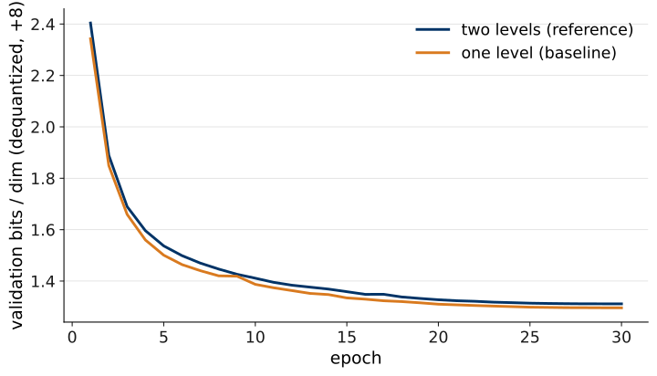
Fresh dequantization noise at every validation; same data, same optimizer, same number of coupling steps. The two-level model evaluates half of its steps at \(7 \times 7\).

Literature numbers are context, not a leaderboard

(Papamakarios, Pavlakou, and Murray 2017, Table 7), MNIST, bits per pixel, fully connected flows: Real NVP (5) \(1.93 \pm 0.01\) · MAF (5) \(1.89 \pm 0.01\) · MADE MoG \(1.41 \pm 0.01\). Same \(\lambda = 10^{-6}\), same \(/256\) (their App. E.2). Glow’s \(3.35\) (Kingma and Dhariwal 2018, Table 2) and RealNVP’s \(3.49\) (Dinh, Sohl-Dickstein, and Bengio 2017, Table 1) are CIFAR-10 — not on this axis.

Exercise. Before placing \(1.300\) next to \(1.93\), list the mismatches: the noise draw · the split · the model class · what the \(\pm\) means · which “logit” (\(\lambda\) vs RealNVP’s \(\alpha = 0.05\) form).

Only the table on the previous slide was produced by one procedure.

06Samples, temperature, honest inspection

TODO 5.1 — \(\tau \in \{0.7, 1.0\}\)

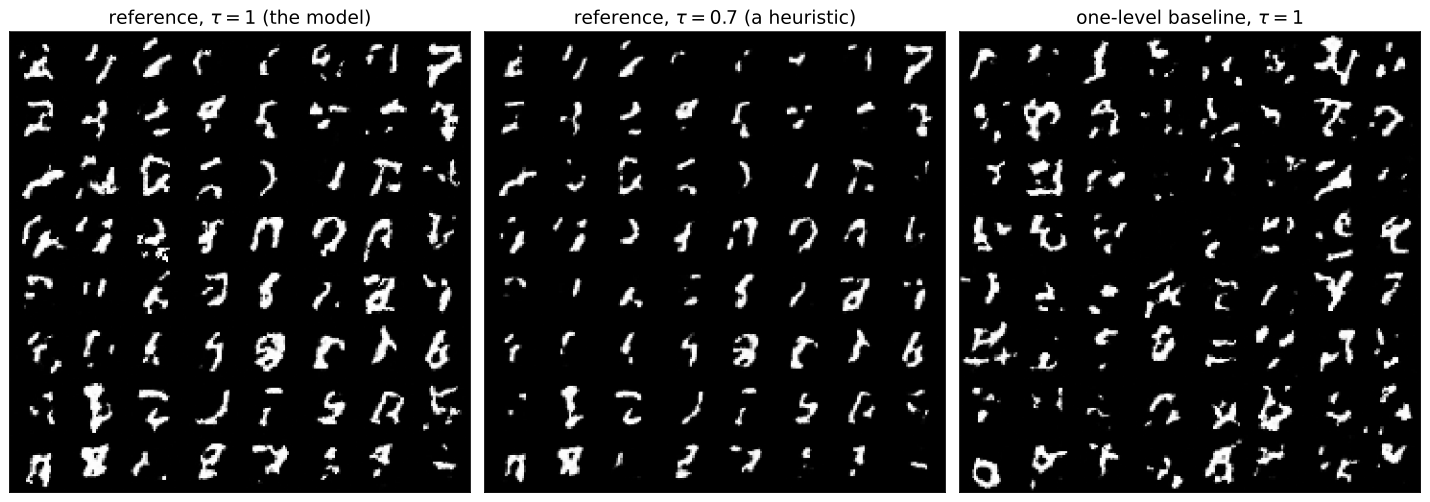
Left: \(\tau = 1\), the model. Middle: \(\tau = 0.7\), a heuristic from a modified base \(\mathcal{N}(0, \tau^2 I)\) — not samples from the model of block E. Right: the baseline at \(\tau = 1\). One noise bank for all three. Fragments of strokes, saturated pixels, speckle: thirty epochs at \(1.300\) bits/dim draw this.

\(\tau \neq 1\) is a heuristic — measured

y = flow.sample(n, tau, generator=g)   # z_l = tau * eps_l
x = logit.forward(y)[0].clamp(0, 1)

The model assigns its own \(\tau = 0.7\) draws a different density than its \(\tau = 1\) draws: -0.451 bits/dim on the sixty-four images of the panel.

Draws the model scores differently from its own samples are, by that measurement, not its samples.

TODO 5.2 — likelihood and samples are different observables

Baseline beside reference, each panel titled with its bits/dim. Then the question, answered only from what you see and measured:

Does the model with the better likelihood produce the better-looking samples? What would you need to say more than “looks”?

(Theis, Oord, and Bethge 2016, sec. 3.2): a model can have poor log-likelihood and great samples, or great log-likelihood and poor samples — constructions in both directions.

The narrow lesson: two observables, neither a proxy for the other. A sample metric is the U3.L2 payoff.

07Close

The two costs, at image scale

Family	Density	Sampling	At image scale
NICE / RealNVP	exact, triangular	direct	conv conditioners; squeeze + factor-out
Glow	exact	direct	two more sums per step
MAF	parallel	sequential	sequential in \(784\)
IAF	sequential	parallel	the same, mirrored
Residual	series log-det	iterative	scales with \(d\); U2.T2

Asymptotics unchanged; the constant changed: 275,040 parameters, 60.5 MFLOP/image, 730 GPU-s.

Two facts you now own

1. An exact likelihood is only meaningful after the observation and dequantization convention is specified. Different \(\lambda\), different bank, no \(+8\) — different number. Under bpd-protocol: \(1.300\).
2. A multi-scale architecture changes bookkeeping and compute, not the change-of-variables theorem. The table of TODO 2.3 is the theorem, summed over a partition — and TODO 4.3 is the trade measured: \(1.49\times\) the arithmetic bought \(0.014\) bits/dim.

The question for U2

A two-level stack accumulates its log-determinant over sixteen coupling steps, each read off one pass. U1.T2 ended with a residual stack whose step size shrinks.

What does the accumulated log-determinant become when the depth becomes continuous?

U2.T1 opens there.

For PS1.4(d) — the cut package

labs/ps1-4d-bundle.npz: sixteen raw uint8 test images, their fixed noise, the checkpoint’s frozen \(\log p_Y\).

With numpy only: \(x = (k+u)/256\) → \(y = T_\lambda(x)\) and its Jacobian → \(\log p_X\) → \(\mathrm{bpd}_{\mathrm{cont}}\) → \(+8\) → compare with \(1.2603\).

No model, no GPU, no \(784\)-dimensional training in the problem set.

What comes next

U2.T1	the residual stack becomes an ODE; the log-determinant becomes an integral of a divergence
U3.T3	an ODE model’s likelihood on MNIST — evaluated under bpd-protocol, this box, these constants
PS1.4(d)	only under the cut rule: the bundle above

References

Dinh, Laurent, Jascha Sohl-Dickstein, and Samy Bengio. 2017. “Density Estimation Using Real NVP.” In International Conference on Learning Representations. https://arxiv.org/abs/1605.08803.

Kingma, Diederik P., and Prafulla Dhariwal. 2018. “Glow: Generative Flow with Invertible \(1 \times 1\) Convolutions.” In Advances in Neural Information Processing Systems. https://arxiv.org/abs/1807.03039.

Papamakarios, George, Theo Pavlakou, and Iain Murray. 2017. “Masked Autoregressive Flow for Density Estimation.” In Advances in Neural Information Processing Systems. https://arxiv.org/abs/1705.07057.

Rozet, François et al. 2022. “Zuko: Normalizing Flows in PyTorch.” https://doi.org/10.5281/zenodo.7625672.

Theis, Lucas, Aäron van den Oord, and Matthias Bethge. 2016. “A Note on the Evaluation of Generative Models.” In International Conference on Learning Representations. https://arxiv.org/abs/1511.01844.