U1.L2 — Multi-Scale Flows on Images
Session U1.L2 · date: see calendar-map
How to read this page. This is the last session of the unit and the first one the calendar cuts if it slips, so the page is written to be read without a lecturer. The previous two sessions built a coupling flow from nothing on points in the plane (U1.L1) and placed it in the zoo of invertible architectures (U1.T2). Today the same algebra meets images: the observations are integers, the dimension is \(784\), and both facts change what a likelihood number means and how the bookkeeping is organized. The contract this session leaves behind is bpd-protocol, a complete convention under which a “bits per dimension” number on MNIST means one thing; U3.T3 evaluates a very different model under it.
These notes are the written record of the lab; the executable part is the notebook labs/lab-u1l2.ipynb (the instructor releases its solutions, lab-u1l2-solutions.ipynb). The page depends on U1.T2 and U1.L1 and on nothing else: where a bootcamp artifact is named, its contract is written out here, and you do not need to have attended the bootcamp.
Four references are optional. (Dinh, Sohl-Dickstein, and Bengio 2017) §3.6 is the multi-scale architecture and §4.1 its preprocessing; (Kingma and Dhariwal 2018) §3 draws the same shell; (Papamakarios, Pavlakou, and Murray 2017) Table 7 and Appendix E.2 are the MNIST numbers and the conversion this page compares itself against; (Theis, Oord, and Bethge 2016) §3.1–3.2 are the two warnings this page turns into protocol. (Rozet et al. 2022) is the library of §3.
Every number on this page was measured. The runs behind the figures and the checkpoints are in scripts/python/fig_u1_l2_multiscale.py, seeded, and the values are recorded in scripts/python/_outputs/u1l2_multiscale.json. The two reference models trained on a GPU, and the JSON says so; every other stage runs on CPU, because the notebook does, and re-running it reproduces the numbers to the digit.
- The
bpd-protocol: observation model, dequantization, preprocessing and evaluation, frozen with their constants in §1. A likelihood number without this box is not a result. - The multi-scale bookkeeping, executable: a squeeze has log-determinant exactly zero, a factor-out is a partition and not a transform, and a per-level table whose rows add up to
log_prob(§2). - A course-internal comparison of two models under one protocol (§4), and the list of reasons a number copied from a paper is not on the same axis.
A fourth thing is deliberately not on the list: a metric for samples. §5 shows that likelihood and samples are different observables, and stops there; the sample metric is the U3.L2 payoff.
0 · Why images change the problem
Block 0 of the lab, 8 minutes.
U1.L1 trained a coupling flow by exact maximum likelihood, and nothing in the algebra depended on \(d = 2\). Two things break when the data become images, and neither of them is the change-of-variables theorem.
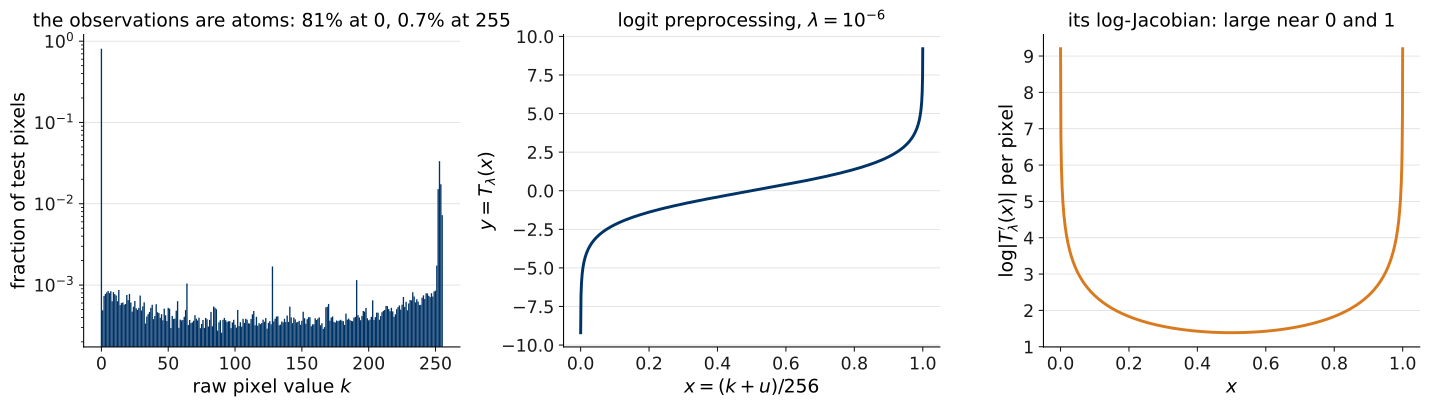
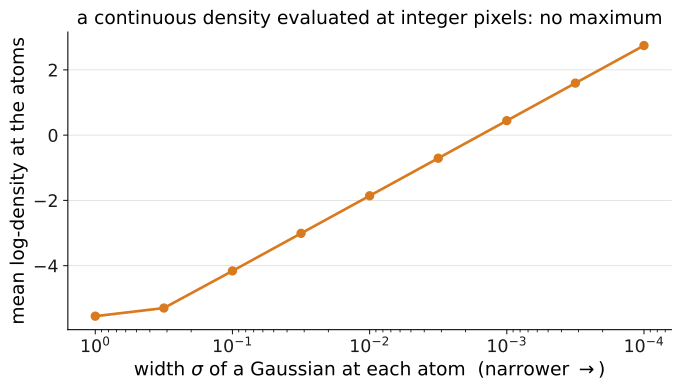
The observations are atoms. An MNIST pixel is stored as an integer \(k \in \{0, \dots, 255\}\). The test set contains exactly 256 distinct values, and 81% of all its pixels are exactly \(0\) (Figure 1, left). A continuous density evaluated at an integer is not a probability mass, and maximizing a continuous density on atoms is ill-posed: the density can grow without bound by concentrating narrower and narrower spikes at the observed integers. Figure 2 computes this for one pixel — a mixture of Gaussians centred at the \(256\) atoms, scored at the atoms, whose mean log-density climbs by 8.3 nats as the width falls from \(1\) to \(10^{-4}\), with no maximum in sight. §1 fixes the observation model before any likelihood is computed.
The dimension is \(784\). A fully connected conditioner on a \(784\)-vector is no longer a toy — the U1.L1 layer at \(d = 784\) with hidden width \(512\) carries about \(0.9\) million parameters per coupling layer — and the log-determinant of a deep stack has to be organized so that it can be read off and checked. §2 is that organization: squeeze, levels of coupling, factor-out.
Given code, and the parity rule
Four modules under common/ arrive as given code. This is the PESC parity rule of L1 §2 in the executable form U1.L1 established: a joint session may consume bootcamp-built artifacts as given code with a contract-level description, and may never require having attended the bootcamp. The bootcamp is provenance, not a prerequisite, and the contract of each module is written here.
| Module | Built in | What this lab uses |
|---|---|---|
common/train.py |
U0.L1, extended in U0.L2 | set_seed; Trainer.fit, exactly as in U1.L1, where the signature is written out |
common/eval.py |
U0.L4 | bpd only (signature in §1); its docstring reserves the dequantization term for “when the course first uses BPD, in U1” — that is this page |
common/coupling.py |
U1.L1 | the affine algebra and HEAD_INIT_SCALE; nothing new |
common/multiscale_flow.py |
today, §2 | Logit, Squeeze2d, ImageAffineCoupling, MultiscaleFlow |
The Trainer is the one of U1.L1: five steps per batch, sched.step() per step, validation under no_grad every epoch, last.pt and best.pt, a CSV log. It expects (x, y) batches and reports an accuracy that reads nan for a flow; that is the interface being preserved. The harness’s bpd takes a vector of per-example log-probabilities in nats and divides by \(d \log 2\); the +8 of §1 is not inside it, on purpose, and the docstring says so.
The data-loader rule
Load MNIST as it is stored: uint8, values in \(\{0, \dots, 255\}\), and keep it that way until the dequantization cell. In particular, keep torchvision.transforms.ToTensor() out: it divides by \(255\), not \(256\), returns floats in \([0, 1]\) with \(255 \mapsto 1\), and hides the factor whose logarithm becomes the \(+8\). The notebook’s Checkpoint 0 loads the raw tensor, asserts its dtype and range, and prints what ToTensor() would have done to it. datasets.MNIST(...).data is the raw tensor.
1 · Dequantization and bits per dimension
Block 1, 18 minutes. Produces the artifact bpd-protocol. Reused in: U3.T3 (the likelihood of an ODE model, evaluated under this box), and PS1.4(d) under the cut rule.
Reference for this section: (Theis, Oord, and Bethge 2016) §3.1, whose equations (3)–(6) are the inequality below in the paper’s scale; (Papamakarios, Pavlakou, and Murray 2017) Appendix E.2 for the conversion to bits; (Papamakarios et al. 2021) §6.1.1 for the vocabulary.
Uniform dequantization, and which way the inequality goes
For a raw pixel vector \(k \in \{0, \dots, 255\}^D\) and \(u \sim \mathrm{Unif}([0,1)^D)\) — the protocol writes the pixel count as \(D\), which is the course’s dimension \(d\), equal to \(784\) here — define
\[ x = \frac{k + u}{256} \in [0, 1)^D . \]
If \(p_X\) is the continuous density the flow models on \([0,1]^D\), the discrete model it induces is the mass of the cell of \(k\), \[ P_\theta(k) = \int_{[k/256,\,(k+1)/256)} p_X(x)\,dx = \frac{1}{256^{D}}\;\mathbb{E}_{u \sim \mathrm{Unif}([0,1)^D)}\!\left[p_X\!\left(\tfrac{k+u}{256}\right)\right], \tag{1}\] by the substitution \(x = (k+u)/256\), whose Jacobian is the constant \(256^{-D}\).
For every \(k\), \[ \log P_\theta(k) = \log \mathbb{E}_{u \sim \mathrm{Unif}([0,1)^D)}\!\left[p_X\!\left(\tfrac{k+u}{256}\right)\right] - D\log 256 \;\ge\; \mathbb{E}_{u \sim \mathrm{Unif}([0,1)^D)}\!\left[\log p_X\!\left(\tfrac{k+u}{256}\right)\right] - D\log 256 . \tag{2}\]
Proof. Take the logarithm of Equation 1; the inequality is Jensen’s, since \(\log\) is concave and \(u \mapsto p_X((k+u)/256)\) is a positive random variable with finite mean. \(\square\)
Read the direction carefully, because both directions get quoted. The quantity a flow is trained on and evaluated with — the expectation of the log-density on dequantized data — is a lower bound on the discrete log-mass, equivalently an upper bound on the discrete negative log-likelihood, in expectation over \(u\). Averaged over the test set, \(-\mathbb{E}[\log P_\theta(k)]\) is the number of nats an entropy code built from \(P_\theta\) would spend per image (Theis, Oord, and Bethge 2016, sec. 3.1); the dequantized objective is at least that. Maximizing the continuous likelihood on dequantized data therefore pushes up a lower bound on the discrete likelihood — which is why training on \(x\) is legitimate at all.
The one-sample estimate is not an exact bound
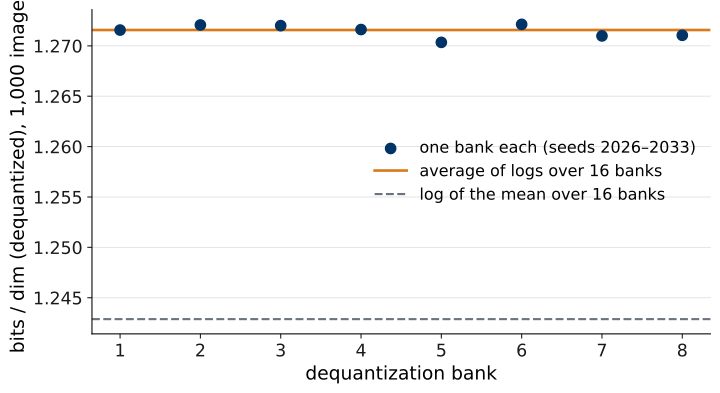
The right-hand side of Equation 2 is an expectation over \(u\). What the notebook computes is a Monte Carlo estimate of it with one draw of \(u\) per image, and a finite estimate fluctuates around the bound value: some draws land above it, some below. Do not call a one-sample realization an exact bound. Figure 3 measures the fluctuation on a fixed \(1{,}000\)-image subset with the reference checkpoint of §4: eight one-sample banks spread over 0.0018 bits per dimension (standard deviation 0.0006), around the sixteen-bank average 1.272; 4 of the eight fall below it. The dashed line is the log of the mean over the sixteen banks, 1.243: a sixteen-sample estimate of the left-hand side of Equation 2 — still a lower bound in expectation, but a tighter one. In nats, Jensen puts the log of the mean never below the average of logs; in bits per dimension the sign flips, and the dashed line is never above the solid one. Several draws per image and a learned dequantization distribution are the publication-grade variants; they are named here and are outside this lab.
Logit preprocessing is a flow layer
A flow on \([0,1]^D\) fights its own boundaries: a Gaussian base pushed through smooth maps puts mass outside the box, and the density near \(x_j = 0\) has to fall to zero in a way coupling layers do not represent well. The standard remedy (Dinh, Sohl-Dickstein, and Bengio 2017, sec. 4.1) is to model the density in logit space.
With \(\lambda = 10^{-6}\), per pixel, \[ a = \lambda + (1 - 2\lambda)\,x, \qquad y = T_\lambda(x) = \operatorname{logit}(a) = \log a - \log(1 - a) . \tag{3}\] \(T_\lambda\) is a bijection of \([0,1]^D\) onto a box in \(\mathbb{R}^D\); its Jacobian is diagonal, so \[ \log\lvert\det J_{T_\lambda}(x)\rvert = \sum_{j=1}^{D}\Big[\log(1-2\lambda) - \log a_j - \log(1 - a_j)\Big] . \tag{4}\]
If the flow models \(p_Y(y)\), the change-of-variables theorem (U1.T1) gives
\[ \log p_X(x) = \log p_Y\big(T_\lambda(x)\big) + \log\lvert\det J_{T_\lambda}(x)\rvert . \tag{5}\]
The preprocessing contribution is never hidden or dropped. In common/multiscale_flow.py the transform is a layer with the course contract: Logit.inverse(x) is the density direction \(x \to y\) and returns Equation 4 as its second output; Logit.forward(y) is the generative direction, \(x = (\sigma(y) - \lambda)/(1 - 2\lambda)\), with the opposite log-determinant written through \(\log\sigma\) so that a large \(\lvert y\rvert\) never produces \(\log 0\). The notebook’s TODO 1.2 writes Equation 4 by hand and checks it against the layer in float64; on a batch of test images the term is about 4620 nats per image, not a rounding error. The flow’s log_prob(y) is \(\log p_Y\); the Jacobian is the caller’s to add, and it stays the caller’s in §4 and in PS1.4(d).
One fine point, for completeness. \(T_\lambda\) maps \([0,1]^D\) onto a bounded box, while \(p_Y\) is a density on all of \(\mathbb{R}^D\); so \(p_X\) integrates over \([0,1]^D\) to the mass \(p_Y\) puts in the box, which is less than \(1\) — a sub-probability density. Every statement on this page holds as written (Jensen needs no normalization, and the coding interpretation becomes “at most this many nats”); the mass beyond \(\lvert y\rvert \approx 13.8\) is negligible for a trained model.
The right-hand side of Figure 1 shows why \(\lambda\) is there: the per-pixel log-Jacobian is large near \(0\) and \(1\), where most MNIST pixels sit, and \(\lambda > 0\) keeps it finite at the endpoints.
Bits per dimension, and the \(+8\)
The eval-harness contract, frozen in U0.L4, is
bpd(log_prob_nats_per_example, num_dims)
    = -mean(log_prob_nats_per_example) / (num_dims * log(2))
and it returns the continuous-density term only. With \(\log p_X\) in nats on \([0,1)^{784}\), the dequantized discrete objective of Equation 2, divided by \(D \log 2\) and read in bits, is
\[ \widehat{\mathrm{bpd}}_{\mathrm{deq}} = \mathrm{bpd}_{\mathrm{cont}} + 8, \qquad \mathrm{bpd}_{\mathrm{cont}} = \frac{-\tfrac{1}{N}\sum_{i=1}^{N}\log p_X(x^{(i)})}{784 \log 2}, \qquad \frac{\log 256}{\log 2} = 8 . \tag{6}\]
The \(+8\) belongs to bpd-protocol, not to the generic harness. Two sanity facts anchor the scale. A uniform density on \([0,1)^{784}\) has \(\log p_X = 0\) and reports exactly \(8\) bits per dimension — the raw 8-bit code, which is what “no model” costs. A model that concentrates has \(\log p_X > 0\) on typical data, so \(\mathrm{bpd}_{\mathrm{cont}}\) is negative and the reported number lands below \(8\): the reference model of §4 has \(\mathrm{bpd}_{\mathrm{cont}} = -6.700\) and reports \(1.300\). The notebook’s Checkpoint 1.3 executes both facts.
The frozen protocol
- raw 8-bit test split; \(D = 784\);
- the full test set, \(N = 10{,}000\), unless a session explicitly labels a CPU-sized diagnostic subset;
- one fixed uniform dequantization noise bank per image,
K_deq = 1, drawn on CPU in test-set order from a generator seeded with \(2026\); - \(\lambda = 10^{-6}\) for the logit transform Equation 3;
- the logit Jacobian Equation 4 is included in \(\log p_X\) before calling
eval_harness.bpd; - reported number:
eval_harness.bpd(log_prob_x, 784) + 8; - every report logs: dataset and split, \(N\), dequantization seed and
K_deq, \(\lambda\), checkpoint hash and configuration.
Publication-grade variants — several \(u\) draws per image, or a learned (variational) dequantization distribution (Papamakarios et al. 2021, sec. 6.1.1) — are named here and are outside this lab.
The bank is fixed so that two evaluations of two models differ because the models differ and not because the noise did; its SHA-256 is recorded in the JSON and asserted by the notebook, so that a torch build whose generator draws differently is detected rather than silently accepted. The checkpoint package of §2 stores these constants beside the weights, and the notebook’s TODO 4.2 logs the report to MLflow with all of them as tags.
U3.T3 evaluates the likelihood of a flow-matching model through an ODE solve and the instantaneous change of variables. Its number is comparable to today’s only if it is computed under this box: same split, same bank, same \(\lambda\), same \(+8\). That is why the box is frozen here, with its constants, and not restated later.
2 · The multi-scale shell
Block 2, 18 minutes. Consumes coupling-layer-scratch (U1.L1). Reused in: U3.T3 (the same shell as the density side of an ODE model’s comparison), U6 seminar on-ramps.
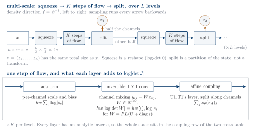
Reference for this section: (Dinh, Sohl-Dickstein, and Bengio 2017) §3.6 (squeeze, factor-out, equations 13–16) and (Kingma and Dhariwal 2018) §3; the picture is from U1.T2 §2, shown again as Figure 4, and this section is its executable bookkeeping.
Three pieces, one contract
common/multiscale_flow.py exposes three pieces you can inspect independently, plus the logit layer of §1. Every one of them has the U1.L1 contract.
# common/multiscale_flow.py — every layer:
#   forward(z) -> (x, logdet_fwd)     # psi   : source -> data
#   inverse(x) -> (z, logdet_inv)     # psi^-1: data -> source
#   logdet_inv == -logdet_fwd, per example, at matching points

Logit(lam=1e-6)                       # inverse = logit (density direction)
Squeeze2d(factor=2)                   # inverse SQUEEZES; both log-dets 0
ImageAffineCoupling(C, mask, hidden)  # U1.L1's layer, mask over CHANNELS,
                                      #   conv conditioner 3x3 -> 1x1 -> 3x3
MultiscaleFlow(in_shape, levels,      # per level: squeeze -> `steps`
               steps, hidden)         #   couplings -> factor out half
    .inverse(y) -> ([z_1, ..., z_L], logdet_inv)
    .forward(zs) -> (y, logdet_fwd)
    .log_prob(y) -> (B,)              # sum_l log p_0(z_l) + logdet_inv
    .sample(n, tau=1.0)               # z_l = tau * eps_l; tau != 1 heuristic
    .bookkeeping(y) -> rows           # one row per level; rows sum to log_prob
Names follow the density direction, as the papers draw it: Squeeze2d.inverse squeezes and MultiscaleFlow.inverse factors out; the generative forward runs every arrow backwards. The coupling layer is the U1.L1 layer with two changes and no new algebra: the mask is a boolean vector over channels, and the conditioner is three convolutions (\(3 \times 3\), \(1 \times 1\), \(3 \times 3\), SiLU between, a small nonzero head for the reason U1.L1 gave), so that \(s\) and \(t\) at a position depend on a neighbourhood of \(x_A\) rather than on all of it. The tanh bound on the log-scale is the same.
Squeeze is a permutation
A squeeze by \(2\) takes each \(2 \times 2\) block of every channel and turns its four entries into four channels at one position: \(1 \times 28 \times 28 \to 4 \times 14 \times 14\). It rearranges the \(784\) entries and touches none of them, so it is a permutation of the coordinates and its log-determinant is exactly \(0\) — not small, zero. The notebook’s TODO 2.1 asserts torch.equal on the round trip and == 0.0 on both log-determinants. (Dinh, Sohl-Dickstein, and Bengio 2017, sec. 3.6) introduce it as “trading spatial size for number of channels”.
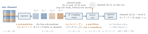
One consequence is worth one sentence, because it decides what the conditioner sees. After a squeeze of a one-channel image, channel \(0\) holds the top-left entry of every block, channel \(1\) the top-right, channels \(2\) and \(3\) the bottom row. A channel mask \(\{0, 1\}\) against \(\{2, 3\}\) is therefore a spatial mask on the original image: the conditioner reads the top row of every \(2 \times 2\) block and moves the bottom row. RealNVP alternates spatial checkerboard masks before a squeeze with channel masks after it (Dinh, Sohl-Dickstein, and Bengio 2017, sec. 3.6, Figure 3); the course shell uses channel masks only, alternated across steps, which is the U1.L1 alternation on a different index.
Factor-out is a partition
At the end of a level, half the channels are sent to the latent collection as they are and the other half continue to the next level at half the resolution. In (Dinh, Sohl-Dickstein, and Bengio 2017, equations 13–16), \[ h^{(0)} = x, \qquad (z^{(l+1)}, h^{(l+1)}) = f^{(l+1)}(h^{(l)}), \qquad z^{(L)} = f^{(L)}(h^{(L-1)}), \qquad z = (z^{(1)}, \dots, z^{(L)}) . \] Factor-out is not an extra Jacobian term. It partitions the current state; nothing is transformed, so nothing is scaled. What \(z_l\) contributes is its base log-probability, and the total is
\[ \log p_Y(y) = \sum_{l=1}^{L} \log p_0(z_l) + \sum_{\text{coupling layers}} \log\lvert\det J_{\psi_k^{-1}}\rvert, \qquad \sum_{l=1}^{L} \dim z_l = 784 , \tag{7}\]
with \(p_0 = \mathcal{N}(0, I)\) on each factor and the second sum taken at the points each layer sees, as in U1.T1 §3. For the reference model, level 1 emits \(z_1\) of shape \(2 \times 14 \times 14\) (\(392\) entries) and level 2 emits \(z_2\) of shape \(8 \times 7 \times 7\) (\(392\) more). The notebook asserts that the latent shapes add up to \(784\) before anything else is done with the model.
Two remarks from the paper, both consequences of the partition. The factors emitted early are “Gaussianized” by fewer layers than the factors emitted late, so the model must make its finer-scale variables Gaussian first (Dinh, Sohl-Dickstein, and Bengio 2017, sec. 3.6) — a statement about representation, not about the theorem. And factoring out early distributes the loss across the stack and halves the number of entries every later layer touches — the paper says “reduces significantly the amount of computation and memory”; the measured version is in §4 and §6.
The bookkeeping table
bookkeeping(y) returns one row per level: the level’s active shape after its squeeze, the sum of its coupling log-determinants, the shape of the factor it emits, and that factor’s \(\log p_0\). There is no squeeze row, because a squeeze contributes nothing. The rows must add up to log_prob(y) per example, and the notebook’s TODO 2.3 asserts that they do.
Batch means over the first sixteen test images, in nats, reference checkpoint of §4:
| level | active shape | coupling log-det | factored latent | base log-prob |
|---|---|---|---|---|
| 1 | \(4 \times 14 \times 14\) | +431.7 | \(2 \times 14 \times 14\) (\(392\)) | -552.7 |
| 2 | \(8 \times 7 \times 7\) | -307.9 | \(8 \times 7 \times 7\) (\(392\)) | -548.3 |
| total | +123.9 | \(784\) | -1101.0 |
Sum of the totals: \(-977.2\) nats \(= \log p_Y\) per image, to a maximum per-example gap of \(1\times10^{-4}\) in float32. Adding the logit term +4639.7 gives \(\log p_X = 3662.5\), and Equation 6 turns it into \(1.2603\) bits per dimension on these sixteen images.
If the table does not add up, a term was counted twice or not at all. In the reference implementation the check passes to \(10^{-14}\) in float64 on the toy shell of the module’s self-test and to float32 rounding on real data; it is the sibling of U1.L1’s per-example Jacobian witness, with exactness in place of automatic differentiation.
Where the other layers would go
The shell is RealNVP-style on purpose. Glow’s step of flow (Kingma and Dhariwal 2018, sec. 3) would insert, before every coupling, an actnorm and an invertible \(1 \times 1\) convolution, each adding the sum U1.T2 §2 wrote for it (\(h w \sum_j \log\lvert s_j\rvert\) and \(h w \log\lvert\det W\rvert\) in PLU form); the shell’s steps list is where they would slot. Neither is needed to make the bookkeeping exact, which is the point of this session, and neither is used.
The live run, and the reference checkpoint’s record
Live training demonstrates the pipeline, not convergence. The notebook’s TODO 2.4 trains a small two-level model (four steps per level, conditioner width \(48\), 50,352 parameters) on \(10{,}000\) training images for three epochs, on CPU, in about 23 s; the reference run measured the held-out number falling from 3.72 to 3.48 bits per dimension. The criterion is pipeline valid and held-out BPD trending downward, not a number to beat. The loss is exact maximum likelihood on dequantized data with the sampling subscripts written out, \[ \mathcal{L}(\theta) = -\,\mathbb{E}_{k \sim q,\; u \sim \mathrm{Unif}([0,1)^D)} \Big[\log p_Y^{\theta}\big(T_\lambda(\tfrac{k+u}{256})\big) + \log\lvert\det J_{T_\lambda}(\tfrac{k+u}{256})\rvert\Big], \tag{8}\] with fresh noise at every step — the fixed bank is for the test report. The Jacobian term does not depend on \(\theta\), so the gradient is the same with or without it; it is kept so that the logged loss converts to bits per dimension by Equation 6 directly.
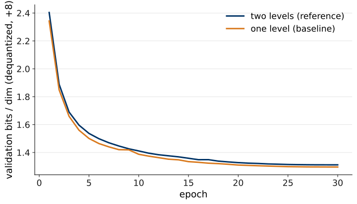
Blocks 4 and 5 read numbers off an instructor-provided checkpoint, and a number read off a checkpoint is only as good as the record that says which code, which data and which settings produced it. The package under common/weights/ therefore stores, beside the weights: the resolved configuration, the seed, the git commit and whether the tree was dirty, the training device and wall-clock, the per-epoch validation curve, the selection rule (last epoch; the test set was never used to select), and the protocol constants of §1. A JSON sidecar carries the file’s SHA-256, and the notebook verifies the hash, the configuration and the constants before loading anything.
| Checkpoint | levels · steps · width | parameters | training | validation bits/dim (last epoch) |
|---|---|---|---|---|
u1l2-multiscale (reference) |
\(2 \cdot 8 \cdot 96\) | 275,040 | 30 epochs, 730 s on NVIDIA GeForce RTX 4070 Laptop GPU | 1.311 |
u1l2-onelevel (baseline) |
\(1 \cdot 16 \cdot 96\) | 233,536 | 30 epochs, 809 s, same GPU | 1.296 |
The baseline is the same conditioner, the same sixteen coupling steps, the same budget, and no factor-out: one squeeze, then all sixteen steps at \(4 \times 14 \times 14\). It isolates the one thing this session adds.
3 · What the library supplies, and what the course shell supplies
Block 3, 12 minutes. Under the cut rule this worksheet becomes U1.L1 TODO 5.3.
Zuko (Rozet et al. 2022) is the course’s reference implementation for discrete flows, and it is used here for exactly what it supplies: the coupling arithmetic, transform composition, and a transform direction to translate. It does not supply a squeeze, a factor-out or a convolutional conditioner — the multi-scale shell is course code, and the worksheet below asks you to say so line by line. As in U1.L1, the source anchors in the notebook are read from the pinned version (zuko 1.5.0) when the notebook is generated, never typed.
Three cross-checks, executed
The notebook runs three checks; each is a numerical identity, not a sentence.
- The logit layer.
zuko.transforms.SigmoidTransform— atorch.distributionsclass Zuko re-exports — is \(y \mapsto \sigma(y)\) with.invthe logit and a log-Jacobian written for the sigmoid direction. OurLogit.inverseis the opposite direction after the affine squeeze into \([\lambda, 1-\lambda]\), so its log-determinant is minus Zuko’s plus \(D\log(1-2\lambda)\). Measured gap in float64: \(9\times10^{-13}\). - The coupling arithmetic.
CouplingTransform(meta, mask)is the skeleton of U1.L1’s layer on a vector: split by the mask, callmeta(x_a)for a transform, apply it tox_b. With the course conv conditioner plugged in asmeta— reshaping the flat vector back to \(2 \times 14 \times 14\) — the library reproducesImageAffineCoupling.inverseand its log-determinant to \(2\times10^{-15}\). Zuko’s_callis the density direction \(f = \psi^{-1}\) (U1.L1 §5), sometareturns the inverse affine map \(x_B = (y_B - t)\,e^{-s}\). - The shell. Nothing in the library squeezes or factors out.
ReshapeTransform(torch’s, re-exported) is a plain reshape with log-determinant \(0\) — the fact about a squeeze without the sub-position permutation — and no transform partitions a state into latent factors. The notebook asserts the absence by name.
The second check is the one to remember. Given the same conditioner, the library and the course produce the same numbers, because the coupling layer is a piece of mathematics and not a piece of software; what the course wrote is the conditioner (an image-scale choice) and the shell (image-scale bookkeeping), and what the library chose is the direction its methods are named in (an API convention).
The worksheet
For each line of the pipeline: model mathematics (a statement of the change-of-variables theorem or of the observation model), image-scale orchestration (bookkeeping that exists because \(d = 784\) is an image), or library API convention (a choice of direction, name or packaging that another library makes differently). The notebook’s TODO 3.4 leaves the two right-hand columns blank; here they are filled.
| Line of the pipeline | Which of the three? | Zuko object, if any |
|---|---|---|
| \(x = (k+u)/256\) | mathematics: the observation model; the \(-D\log 256\) of Equation 2 | none — dequantization is the caller’s |
| \(y = T_\lambda(x)\) and Equation 4 | mathematics: a flow layer with its change-of-variables term | SigmoidTransform (torch’s, re-exported), opposite direction, no \(\lambda\) |
| \(y_B = x_B e^{s} + t\), log-det \(\sum s\) | mathematics: U1.T1 §5, on a vector or on a feature map | CouplingTransform + AffineTransform |
| the conv conditioner \(s, t = c_\theta(x_A)\) | orchestration: locality; a vector MLP would carry \(784\times\) width parameters per layer | the meta slot exists (an MLP hypernetwork); the conv does not |
| squeeze | orchestration: a permutation, log-det \(0\) | ReshapeTransform (torch’s), a reshape only |
| factor-out of channels \(\{0,1\}\) as \(z_1\) | orchestration: a partition, no Jacobian term | none |
| Equation 7 | mathematics: the theorem, summed over a partition | Flow.log_prob sums the same objects for one latent |
forward is \(\psi\); Zuko’s _call is \(\psi^{-1}\) |
API convention: \(f = \psi^{-1}\) (U1.L1 §5) | LazyTransform, transform() |
bpd(log_prob_x, 784) + 8 |
mathematics: the observation model in bits — and a course convention on where the \(+8\) lives | none |
4 · The checkpoint under the frozen protocol
Block 4, 14 minutes.
The reported number
The notebook’s TODO 4.1 computes \(\log p_X\) for the full test set with the fixed bank, in chunks of \(500\) under no_grad, Jacobian included; on a laptop core the \(10{,}000\) images take about 14 s. TODO 4.2 calls the protocol, checks it against the manual arithmetic on a fixed batch of sixteen (Table 2), and logs the report to MLflow with the protocol constants as tags. TODO 4.3 does the same for the baseline with the same bank, the same \(\lambda\), the same \(N\).
bpd-protocol on the full test set, \(N = 10{,}000\), bank seed \(2026\), \(\lambda = 10^{-6}\), one seed of each model.
| Checkpoint | parameters | \(\mathrm{bpd}_{\mathrm{cont}}\) | reported \(\widehat{\mathrm{bpd}}_{\mathrm{deq}}\) |
|---|---|---|---|
u1l2-multiscale (two levels) |
275,040 | \(-6.700\) | \(1.300\) |
u1l2-onelevel (baseline) |
233,536 | \(-6.714\) | \(1.286\) |
The gap is \(0.014\) bits per dimension in favour of the one-level model. A paired bootstrap over the shared test images — the same \(k\), the same \(u\) for both models, \(2{,}000\) resamples — puts the 95% interval of the difference (one-level minus two-level) at \([-0.015,\ -0.014]\): the gap is larger than test-set sampling noise. It is still one training seed of each model, and a seed spread is not on this page.
The gap has a price. “The same number of coupling steps” is not “the same compute” when half of one model’s steps run at \(7 \times 7\): one density evaluation costs 90.3 MFLOP per image for the one-level model against 60.5 for the two-level one, a factor of 1.49, counted by torch.utils.flop_counter; the training runs took 809 against 730 GPU-seconds. The one-level model bought its \(0.014\) bits per dimension with half again as much arithmetic.
This is the quantitative comparison the protocol allows you to interpret directly: the two numbers were produced by one measurement procedure, so their difference is a statement about the two models and nothing else. What it says is the honest version of the multi-scale trade: at matched steps and epochs, factoring out half the state after eight steps costs a little likelihood and buys a third of the compute. The shell of §2 changes bookkeeping and compute, not the theorem — and not, by itself, the number. Figure 6 shows the validation curves that produced the two checkpoints.
Literature numbers are context, not a leaderboard
(Papamakarios, Pavlakou, and Murray 2017, Table 7) report MNIST in bits per pixel for fully connected flows: Real NVP with five coupling layers \(1.93 \pm 0.01\), MAF (5) \(1.89 \pm 0.01\), MADE MoG \(1.41 \pm 0.01\). Their Appendix E.2 converts from nats in logit space (their Table 2, where Real NVP (5) is \(-1323.2 \pm 6.6\)) with the same \(\lambda = 10^{-6}\) and the same division by \(256\) — which is why the course uses this form of the transform. Glow reports no MNIST number at all; its \(3.35\) bits per dimension (Kingma and Dhariwal 2018, Table 2) and RealNVP’s \(3.49\) (Dinh, Sohl-Dickstein, and Bengio 2017, Table 1) are CIFAR-10, a different dataset, and not on this axis.
Before placing today’s \(1.300\) next to their \(1.93\), the exercise asks for the list of protocol mismatches. The reference list:
- the paper does not say how the test-time noise was drawn, fixed or fresh; ours is a fixed bank with a recorded hash — a difference inside the fluctuation of §1, but an unknown one;
- their split holds out \(10{,}000\) training images for validation; ours holds out \(5{,}000\);
- their models are fully connected flows on the \(784\)-vector with five or ten coupling or autoregressive layers; ours are convolutional and multi-scale — so a gap between the numbers mixes architecture with everything above;
- their \(\pm\) is “2 standard deviations” in the caption, which the numbers show to be two standard errors of the test-set mean under one model (\(\pm 6.6\) nats over \(10{,}000\) images cannot be two per-image standard deviations of a \(784\)-dimensional log-likelihood), not a spread across training seeds; neither number carries a seed spread;
- the term “logit preprocessing” names two different transforms: (Papamakarios, Pavlakou, and Murray 2017) and this course use Equation 3, with \(\lambda\), while RealNVP’s own paper uses \(\operatorname{logit}(\alpha + (1-\alpha)\,x)\) with \(\alpha = 0.05\) on all of its datasets (Dinh, Sohl-Dickstein, and Bengio 2017, sec. 4.1).
Only Table 5 was produced by one procedure. It is the comparison you may read as a statement about the models, and even it is one seed of each.
5 · Samples, temperature, and an honest inspection
Block 5, 12 minutes.
Sampling at \(\tau \in \{0.7, 1.0\}\)
MultiscaleFlow.sample(n, tau) draws \(z_l = \tau\,\varepsilon_l\) with \(\varepsilon_l \sim \mathcal{N}(0, I)\) per factor, runs the generative direction, and returns \(y\) in logit space; Logit.forward takes it back to \([0,1]\). At \(\tau = 1\) these are samples from the model whose likelihood §4 reported. At \(\tau = 0.7\) they are not: they are draws from a modified base \(\mathcal{N}(0, \tau^2 I)\) pushed through the same map — a sampling heuristic, and every panel at \(\tau \neq 1\) is labelled as one. One fixed noise bank serves both panels, so that they differ by \(\tau\) only.
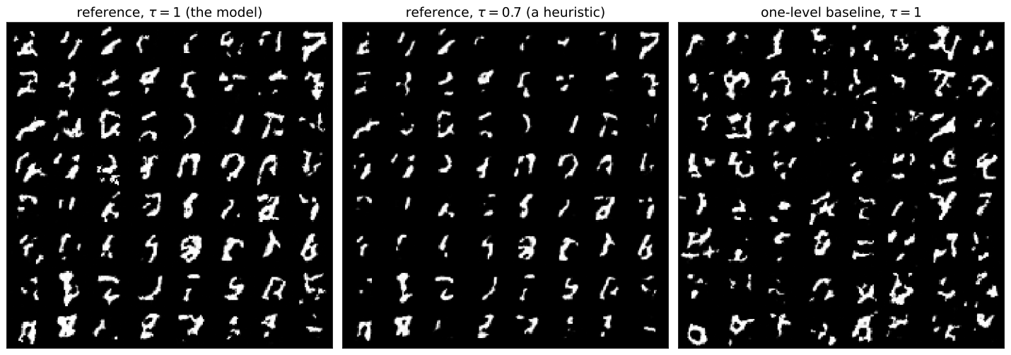
What the panels show, before any number is attached: strokes and fragments of digits, with nearly every pixel at \(0\) or \(1\) and a speckle of isolated pixels in the background. The saturation is the logit map: a model in \(y\)-space that puts mass at \(\lvert y\rvert > 5\) produces pixels within \(10^{-2}\) of the boundary, which is where 81% of MNIST lives; the speckle is mass the model leaves in the stretched region near \(x = 0\), where Figure 1’s log-Jacobian is largest. Thirty epochs of a \(275{,}040\)-parameter flow at \(1.300\) bits per dimension draw this; a longer run and a wider conditioner draw cleaner strokes at a lower number, and neither is the point of the block.
One measured fact keeps the label honest. The model assigns its own \(\tau = 0.7\) draws a different density than its \(\tau = 1\) draws: -0.451 bits per dimension (\(\tau{=}0.7\) minus \(\tau{=}1\)), measured on the sixty-four images of Figure 7. Draws that the model scores differently from its own samples are, by that measurement, not its samples; they are a different distribution, related to the model by a choice someone made.
Likelihood and samples are different observables
Put the baseline’s \(\tau = 1\) panel beside the reference’s, each with its bits per dimension in the title, and ask whether the model with the better likelihood produces the better-looking samples. The one-level model has the lower number, by a margin the paired bootstrap places away from zero. To this author’s eye its panel is the more fragmented of the two — more broken strokes, more isolated pixels — which is the opposite ordering from the likelihood; a second reader may order the panels differently, and the likelihood gap does not move while they argue. (Theis, Oord, and Bethge 2016, sec. 3.2) give constructions in both directions — a lookup table of training images with excellent samples and poor test likelihood, and a mixture that scores well and draws poorly — and their sentence is the lesson: a model can have poor log-likelihood and produce great samples, or great log-likelihood and poor samples.
The narrow conclusion, and only this: an exact likelihood and the visual quality of samples are different observables of the same model, and neither is a proxy for the other. To say more than “looks”, one needs a measurement protocol for samples — an extractor, a reference set, a sample count, and the caveats that come with them. That protocol is the U3.L2 payoff; it is not introduced here.
6 · Close: what an exact likelihood buys, and costs
Block 6, 8 minutes.
The two costs, at image scale
The persistent board of the unit is U1.T1’s table, extended to version 2 in U1.T2 §8. Here it is once more, with one annotation per row for what image scale did to it today.
| Family | Density / likelihood | Sampling | At image scale |
|---|---|---|---|
| NICE / RealNVP | exact: analytic inverse, triangular log-det | direct | conditioners become convolutions; squeeze and factor-out keep the stack tractable in parameters and memory (Dinh, Sohl-Dickstein, and Bengio 2017, sec. 3.6) |
| Glow | exact | direct | actnorm and \(1 \times 1\) convolutions slot into each step; two more sums per step (U1.T2 §2) |
| MAF | parallel density, sequential sampling | sequential in \(784\): the cost that kept the fully connected MNIST flows of Table 7 at five or ten layers | |
| IAF | sequential density | parallel sampling | the same, mirrored |
| Residual flow | direct map; log-det a stochastic series | iterative inverse | the series and the estimator scale with \(d\); U2.T2 |
The “cheap” coupling construction is cheap in the sense of U1.T1: no determinant is formed, the inverse is analytic. It is not cheap in absolute compute: 275,040 parameters, 60.5 MFLOP per density evaluation and 730 GPU-seconds for one number on MNIST, and the two-level shell exists precisely to cut the cost of every step after the first factor-out — a level-2 step costs about a third of a level-1 step here, by the FLOP count. Table 5 is that trade measured: the one-level model, at 1.49 times the arithmetic per image, reached a likelihood \(0.014\) bits per dimension better. Every bit of either number is exact, which is what the unit paid for.
Two facts you now own
- An exact likelihood is only meaningful after the observation and dequantization convention is specified. The same checkpoint reports a different number under a different \(\lambda\), a different bank, or without the \(+8\); it reports \(1.300\) under
bpd-protocol, and U3.T3’s number will be read under the same box. - A multi-scale architecture changes bookkeeping and compute, not the change-of-variables theorem. Table 2 is the theorem, summed over a partition, and its rows add up.
The question for U2
A two-level stack accumulates its log-determinant over sixteen coupling steps, each read off one pass. U1.T2 §7 ended with a residual stack whose step size shrinks. What does the accumulated log-determinant become when the depth becomes continuous? — U2.T1 opens there.
Reading the board
The two boards of the live session, in case you were not there.
- Board 1 holds the dequantization inequality Equation 2 and the derivation of the \(+8\) from Equation 6, and stays visible through the evaluation block: every number of §4 is read against it.
- Board 2 is Figure 5: the squeeze as a permutation with “log-det \(= 0\)” written beside it, and the factor-out with “a partition, not a transform”.
For PS1.4(d)
Under the cut rule, this session’s protocol becomes part (d) of PS1.4, as a CPU bookkeeping exercise on provided outputs and never as \(784\)-dimensional training. The package is labs/ps1-4d-bundle.npz: sixteen raw uint8 test images, their fixed dequantization noise from the bank of §1, and the reference checkpoint’s frozen \(\log p_Y\) at the corresponding \(y\). With numpy only, reconstruct \(x = (k+u)/256\), \(y = T_\lambda(x)\) and Equation 4, then \(\log p_X\) by Equation 5, then \(\mathrm{bpd}_{\mathrm{cont}}\) and the \(+8\) by Equation 6, and compare with the value recorded in the bundle, \(1.2603\). The notebook’s TODO 6.1 is the same exercise with the answer beside it.
Where this page reappears
| Artifact | Section | Consumed by |
|---|---|---|
bpd-protocol |
§1 | U3.T3 (ODE-model likelihood, same box); PS1.4(d) under the cut rule |
| the multi-scale bookkeeping Equation 7 | §2 | U3.T3 (the density side of the comparison); U6 on-ramps |
| the checkpoint package and its record | §2 | any later session that quotes a likelihood on MNIST |
two-costs-table v2, annotated |
§6 | U2.T2 (v3), U3.L1 |
Next session
U2.T1 opens the continuous-time unit: the residual stack of U1.T2 §7 becomes an ODE, the accumulated log-determinant becomes an integral of a divergence, and the two costs of the board are rewritten for a map that no architecture constrains. Nothing about the observation model changes: when U3.T3 evaluates an ODE model on MNIST, it does so under §1.