U1.T2 — The Zoo and Its Limits
Session U1.T2 · date: see calendar-map
How to read this page. This is the closing theory session of the unit, and it pays three debts. U1.T1 left two questions on its board without an answer: how expressive a stack of coupling layers is (the depth question), and what the three hypotheses of the change-of-variables theorem cost (the fine print). U1.L1 added an observation without an explanation: a RealNVP trained on the gapped checkerboard put \(29.8\%\) of its mass where the data density is exactly zero, and stopped half a nat short of the entropy of the data. This page opens the rest of the discrete-flow zoo, answers the depth question with one positive result and one negative one, explains the checkerboard, and ends on the doorstep of continuous time.
These notes are written to be read on their own. They depend on U1.T1, on U1.L1 (for the checkerboard evidence, which is quoted here in full), and on UP.T1. You do not need to have attended the bootcamp. Where a bootcamp artifact is named, the thing it names is written out here.
Two references cover the zoo at book length and both are optional: (Papamakarios et al. 2021) (its §3.1 is the autoregressive family, §3.3.1 the residual family, §2.2 the expressivity question) and (Bishop and Bishop 2024) ch. 18. The original papers are cited section by section below; two of them, (Cornish et al. 2020) and (Draxler et al. 2024), are the modern sources for the limits in §4 and §5, and this page states their results with the hypotheses attached.
- The depth question (U1.T1 §6). How expressive is a stack of coupling layers, really? — §4.
- The fine print (U1.T1 §2). A flow is a diffeomorphism of \(\mathbb{R}^{d}\). What can a diffeomorphism not do? — §5.
- The checkerboard gaps (U1.L1 §4). Why did the model put mass in the gaps, and is that a theorem or an accident? — §5.
The live session keeps all three on the board, and Section 9.1 reads them off at the end.
§1 — Where the unit stands
Reference for this section: U1.T1 §3 and U1.L1 §4, restated without proof.
The two costs, version 1
U1.T1 fixed the direction convention of the unit: the generative map is \(\psi^{\theta} \colon z \to x\), sampling runs it forward, and density evaluation runs \((\psi^{\theta})^{-1}\) and needs \(\log\lvert\det
J_{\psi_k}\rvert\) for every layer on the way. Those two requirements are the two rows of the two-costs-table (U1.T1, box “The two costs (v1)”), and the unit’s thesis is one sentence: the architectural zoo is a list of tricks to make both rows cheap at once. This page fills the table with the rest of the zoo and rewrites it as version 2 in Section 8.
Two facts from U1.T1 are used throughout, both without proof:
- a flow is a composition \(\psi = \psi_K \circ \cdots \circ \psi_1\) of diffeomorphisms, and its log-likelihood telescopes into a sum of per-layer log-determinants (U1.T1 §3);
- an affine coupling layer has a block-triangular Jacobian, so \(\log\lvert\det J\rvert = \sum_j s_\theta(x_A)_j\), a sum read off one forward pass, and an inverse that is analytic (U1.T1 §5).
The checkerboard evidence
U1.L1 trained a six-layer RealNVP on the gapped checkerboard of its toy2d-datasets: eight separated squares of side \(1.5\), no jitter, and exactly zero density between them. The dataset contract matters for everything in §5, so here it is again: of \(100{,}000\) generated points, \(0\) fall outside the eight squares. The trained model is shown in Figure 1, which is U1.L1’s figure reused unchanged.
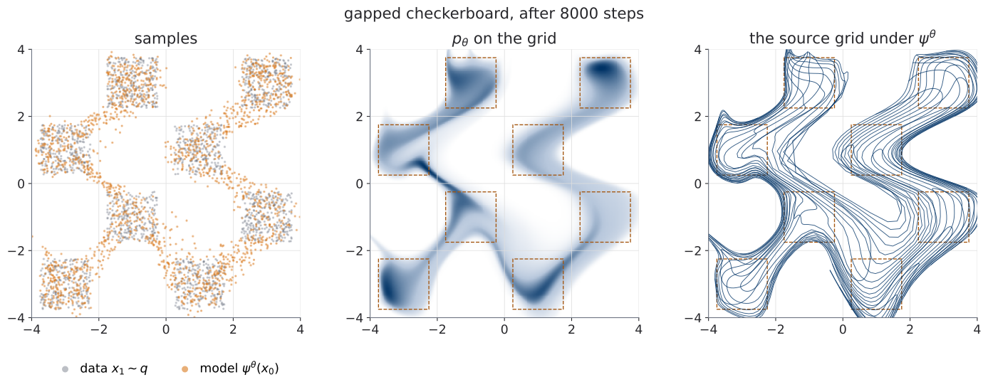
The lab measured four numbers on this model and explained none of them:
| Measured in U1.L1 §4 | Value |
|---|---|
| model mass outside the eight squares | \(29.8\%\) |
| mean model density in the gaps, relative to the mean on the support | \(0.166\) |
| minimum model density on the segment between two diagonal neighbours | \(0.040\), against \(1/18 \approx 0.056\) inside a square |
| validation NLL, against the entropy \(\log 18 = 2.890\) nats of the data | \(3.39\) nats, \(0.50\) above |
The checkerboard is the unit’s controlled witness. It returns as the same points under other models in U2.L1, U2.L2, U3.L1 and U3.L3, and the separation drawn in §5 between what a diffeomorphism cannot do and what a finite model happened not to do is reused as a debugging aid in the final-project workshop (U7.W1).
§2 — Glow: the coupling family at image scale
Reference for this section: (Kingma and Dhariwal 2018) §3 and its Table 1. Glow is not a new theorem. It is the affine coupling layer of U1.T1, engineered for \(32 \times 32\) and \(256 \times 256\) images, with two extra layer types whose log-determinants are as cheap as coupling’s. Both are worth knowing because both are read off in one line.
Actnorm
Deep coupling stacks are hard to train from a random initialization, and the first RealNVP used batch normalization for it. Glow’s stated reason to drop it is practical: the noise batch normalization adds grows as the per-device minibatch shrinks, and Glow trains large images at one image per device (Kingma and Dhariwal 2018, sec. 3.1). A reason this course adds: batch normalization has two states, train and eval, and its train-time output depends on the whole minibatch, a poor fit for a model whose density must be a function of one input. Glow replaces it by actnorm: a per-channel affine transformation. On an \(h \times w \times c\) feature map with channel scale \(s \in \mathbb{R}^{c}\) and bias \(b \in \mathbb{R}^{c}\), \[ \begin{aligned} y_{ij} &= s \odot x_{ij} + b \quad\text{for every spatial position } (i,j), \\ x_{ij} &= (y_{ij} - b) / s . \end{aligned} \tag{1}\]
The Jacobian of the layer as displayed, \(x \mapsto y\), is diagonal, with each channel’s \(s_j\) repeated once per spatial position, so \[ \log\lvert\det J\rvert = h\,w \sum_{j=1}^{c} \log\lvert s_j\rvert . \tag{2}\]
Both formulas of this section are written for the layer in the direction displayed; read for the generative map \(\psi\) they change sign, as §3, MAF spells out for the autoregressive case, and as U1.T1 §3 did for coupling.
Data-dependent initialization is not batch normalization. Actnorm’s \(s\) and \(b\) are initialized so that the first minibatch comes out with zero mean and unit variance per channel (Kingma and Dhariwal 2018, sec. 3.1). After that step they are ordinary parameters: no batch statistics, no train/eval split, one function of one input. Invertibility needs \(s_j \neq 0\) for every channel, which the initialization guarantees and training preserves in practice.
The invertible \(1 \times 1\) convolution
U1.T1 §6 alternated masks or inserted fixed permutations so that every coordinate is eventually moved. Glow learns the permutation. A \(1 \times 1\) convolution with \(c\) input and \(c\) output channels applies one matrix \(W \in \mathbb{R}^{c \times c}\) at every spatial position, \[ y_{ij} = W x_{ij}, \qquad \log\lvert\det J\rvert = h\,w\,\log\lvert\det W\rvert , \tag{3}\]
and a permutation is the special case where \(W\) is a permutation matrix (Kingma and Dhariwal 2018, sec. 3.2). The determinant of a dense \(c \times c\) matrix costs \(O(c^{3})\), which is a cost per layer, not per data point, and is often comparable to the \(O(h w c^{2})\) of applying the mixing itself. Glow removes it anyway, by parameterizing \(W\) in its PLU form, \[ W = P\,L\,(U + \operatorname{diag}(s)), \qquad \log\lvert\det W\rvert = \sum_{i=1}^{c} \log\lvert s_i\rvert , \tag{4}\]
with \(P\) a fixed permutation, \(L\) lower-triangular with unit diagonal, \(U\) strictly upper-triangular, and \(s \in \mathbb{R}^{c}\) learned. The determinant bookkeeping is now \(O(c)\); the dense channel mixing still costs \(O(h w c^{2})\) to apply, PLU or not. Invertibility needs \(s_i \neq 0\) for every \(i\).
Take a \(32 \times 32 \times 12\) feature map, the shape after Glow’s first squeeze of a \(64 \times 64 \times 3\) image. Actnorm has \(24\) parameters and its log-determinant is \(1024 \sum_{j=1}^{12} \log\lvert s_j\rvert\): twelve logarithms, one sum. The \(1 \times 1\) convolution has \(144\) parameters; applying it costs \(1024 \times 144\) multiply-adds, its log-determinant in PLU form is \(1024 \sum_{i=1}^{12} \log\lvert s_i\rvert\), twelve logarithms again. Neither layer forms a Jacobian. Both sit in the same row of the two-costs table as coupling: analytic inverse, log-determinant read off.
The multi-scale picture
One picture and no implementation: U1.L2 owns the executable bookkeeping. Glow processes an image at several resolutions. A level squeezes the tensor (a reshape from \(h \times w \times c\) to \(\frac{h}{2} \times \frac{w}{2} \times 4c\), log-determinant zero), applies \(K\) steps of flow, and splits: half of the channels are sent straight to the latent as \(z_l\), the other half go down to the next level at half the resolution. A step of flow is actnorm, then the \(1 \times 1\) convolution, then affine coupling split along channels. Figure 2 draws it.
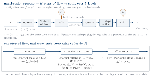
Two bookkeeping facts to hold on to, both examined in U1.L2: squeeze is a reshape, so it contributes nothing to the log-determinant; and split is a partition of the state, not a transform, so it contributes nothing either. The total \(z\) has the same size as \(x\).
| Density / likelihood | Sampling | |
|---|---|---|
| Glow | exact: coupling sums \(+\) actnorm sums \(+\) PLU sums, per position | direct: every layer has an analytic inverse |
Glow is the coupling row of the table, engineered for images. It adds no new theorem and removes no limitation of §4 and §5.
§3 — Autoregressive flows: MAF and IAF
Reference for this section: (Papamakarios, Pavlakou, and Murray 2017) §3, (Kingma et al. 2016) §3–4, and (Papamakarios et al. 2021) §3.1 for the general form. This is the second family of the zoo, and it is where the two costs come apart most cleanly.
The autoregressive factorization
Any density on \(\mathbb{R}^{d}\) factorizes by the chain rule. Writing the coordinates of a point as \(x = (\xi_1, \dots, \xi_d)\), \[ p(x) = \prod_{i=1}^{d} p(\xi_i \mid \xi_{<i}), \qquad \xi_{<i} = (\xi_1, \dots, \xi_{i-1}) . \tag{5}\]
A model that parameterizes each factor by a network reading only earlier coordinates has an exact likelihood, and this is the whole design of the autoregressive family. (PGMAT heard this sentence in U0.T3’s panorama; it is stated here in full and nothing below depends on that session.) The coordinate notation is deliberate: in this course \(x_1\) is a data point, never a coordinate, so a coordinate is \(\xi_i\) and the coordinates of a source point \(z\) are \(\zeta_i\).
MAF: the density transform
Fix the coordinates of the source point \(z = (\zeta_1, \dots, \zeta_d)\). A masked autoregressive flow parameterizes the density transform \(f = \psi^{-1} \colon x \to z\) coordinate by coordinate, \[ \zeta_i = \frac{\xi_i - \mu_i(\xi_{<i})}{\sigma_i(\xi_{<i})}, \qquad \sigma_i > 0, \tag{6}\]
with \(\mu_i, \sigma_i\) produced by one masked network that reads \(\xi_{<i}\) — a network whose weight masks let output \(i\) depend on inputs \(1, \dots, i-1\) only — (Papamakarios, Pavlakou, and Murray 2017, sec. 3, eq. 4). The paper writes \(\alpha_i = \log\sigma_i\); the translation is silent, per the notation standard. The Jacobian of \(f\) is triangular with diagonal \(1/\sigma_i\), so in course form, for the generative map at \(z = f(x)\), \[ \log\lvert\det J_{\psi}(z)\rvert = \sum_{i=1}^{d} \log\sigma_i(\xi_{<i}) . \tag{7}\]
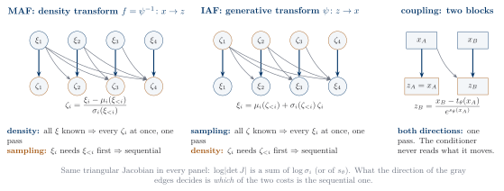
Density is one pass. At density time every \(\xi_i\) is known, so the masked network produces all \((\mu_i, \sigma_i)\) in parallel and Equation 6 gives every \(\zeta_i\) at once. Sampling is sequential. Given \(z\), the inverse recursion \(\xi_i = \mu_i(\xi_{<i}) + \sigma_i(\xi_{<i})\,\zeta_i\) needs \(\xi_{<i}\) before it can produce \(\xi_i\): coordinate by coordinate, in the event dimension, the \(d\) coordinates of one point.
IAF: the generative transform
An inverse autoregressive flow parameterizes the generative map \(\psi \colon z \to x\) instead, with the conditioner reading the source coordinates, \[ \begin{aligned} &\xi_i = \mu_i(\zeta_{<i}) + \sigma_i(\zeta_{<i})\,\zeta_i, \\ &\log\lvert\det J_{\psi}(z)\rvert = \sum_{i=1}^{d} \log\sigma_i(\zeta_{<i}) . \end{aligned} \tag{8}\]
(Kingma et al. 2016, secs. 3–4.) Sampling is one pass: every \(\zeta_i\) is known, so all \((\mu_i, \sigma_i)\) come out in parallel and so does every \(\xi_i\). Density evaluation is sequential: given an external \(x\), recovering \(\zeta_i = (\xi_i - \mu_i(\zeta_{<i})) / \sigma_i(\zeta_{<i})\) needs \(\zeta_{<i}\) first.
Duality, stated carefully
Equation 6 and Equation 8 look like the same formula read in opposite directions, and it is tempting to say that MAF and IAF are “the same map”. They are not. In MAF the conditioner reads the data coordinates \(\xi_{<i}\); in IAF it reads the source coordinates \(\zeta_{<i}\). These are different parameterized families — “different models with different computational trade-offs”, in the words of (Papamakarios, Pavlakou, and Murray 2017, sec. 3.2). What the two families share is a triangular dependency structure, and what distinguishes them is the direction of that dependency, which decides which of the two costs is the sequential one. Figure 3 draws both, with a coupling layer beside them.
| Family | Density / likelihood | Sampling |
|---|---|---|
| MAF | parallel, one pass | sequential inverse, in the event dimension |
| IAF | sequential inverse, in the event dimension | parallel, one pass |
The phrase “\(d\) passes” for the sequential direction is an intuition for affine scalar autoregression, where each coordinate needs one more evaluation of the conditioner. The implementation-level statement is “sequential in the event dimension”; it is not a promise about an exact count of network calls, which depends on caching and on the conditioner’s architecture.
Coupling is block-autoregressive
Put two blocks in place of \(d\) coordinates: \(x = (x_A, x_B)\), the first block copied, \(z_A = x_A\), and the second transformed conditionally on the first, \(z_B = (x_B - t_\theta(x_A)) \odot e^{-s_\theta(x_A)}\). This is U1.T1’s affine coupling layer, and it is an autoregressive map with two blocks (Papamakarios et al. 2021, sec. 3.1.2). The conditioner never reads what it moves, so both directions are one pass, and that is exactly why coupling gave up something: a single coupling layer cannot represent an arbitrary autoregressive transformation, and the price is paid in depth, with permutations between layers so that every coordinate is eventually moved (U1.T1 §6). The zoo is unified: coupling, MAF and IAF are the same triangular idea at different block sizes and in different directions.
The task-direction table is the reading key for every library cross-check of the course. A library that exposes MAF-style transforms parameterizes \(f = \psi^{-1}\), and U1.L1’s direction table applies unchanged. U2 keeps the triangular idea out of the picture entirely: its maps have dense Jacobians and pay for the log-determinant in a different currency.
§4 — Universality, and its fine print
Reference for this section: (Draxler et al. 2024) §4–5 for the two anchors, (Papamakarios et al. 2021) §2.2 and §3.1.2 for the classical context. This section answers the depth question, and the answer has two halves.
The negative anchor: volume-preserving flows
NICE’s additive coupling layers have unit determinant (U1.T1 §4), and so does any stack of them: a volume-preserving flow. U1.T1 §4 stated the limitation as the inability to change local volume, and its Exercise 2 deferred the question of whether NICE’s final scaling layer makes a target reachable. The modern statement answers it.
The family of normalizing flows with constant Jacobian determinant \(\lvert\det J_{\psi}\rvert = \text{const}\) is not a universal distribution approximator under KL divergence. Moreover, a flow built from diffeomorphisms with constant Jacobian determinant has the same number of modes as its base distribution.
The second sentence is the one to remember. A constant-Jacobian diffeomorphism maps a neighbourhood of a density maximum to a neighbourhood of a density maximum, because the density values are all multiplied by the same constant; so a unimodal base gives a unimodal model, and no depth changes that (Draxler et al. 2024, sec. 4, proof in its App. B.3). The authors also quantify the loss: for a standard normal base and a continuous bounded target, the achievable KL is bounded below by an explicit nonnegative number depending on the target (their Theorem 4.1). NICE’s final scaling layer does not help. Its determinant is the product of its diagonal entries — a constant, independent of the input — so additive coupling plus a scaling layer is still a constant-determinant flow, and Theorem 4.2 and Proposition 4.3 apply to it exactly as without the layer. That is the answer to U1.T1’s Exercise 2. What removes the obstruction is a layer whose determinant varies with the input: RealNVP’s \(e^{s_\theta(x_A)}\).
The positive anchor: affine coupling flows
The classical argument is constructive and goes through the autoregressive form of §3, but it needs more than affine layers. For any target with a density that is positive everywhere and whose conditional distribution functions are differentiable, there is a triangular diffeomorphism that maps it to the uniform distribution on \((0,1)^{d}\) — the map whose \(i\)-th coordinate is the conditional CDF of \(\xi_i\) given \(\xi_{<i}\) (Papamakarios et al. 2021, sec. 2.2). An autoregressive flow can represent that map when both its conditioners and its transformers are flexible enough (Papamakarios et al. 2021, sec. 3.1), and \(d\) coupling layers with the right splits can represent any autoregressive map (Papamakarios et al. 2021, sec. 3.1.2). The affine transformer of §3 is not flexible enough: for fixed \(\xi_{<i}\) it is an affine function of \(\xi_i\), and an affine function is not a conditional CDF. So the classical argument says nothing about RealNVP, which is why the affine case needed a theorem of its own. That theorem is recent, and its convergence notion and hypotheses are part of the statement.
Let \(p\) be a continuous density on \(\mathbb{R}^{d}\) with finite first and second moments and infinite support. Then there is a sequence of flows \(f_n\), each a composition of \(n\) affine coupling blocks that are \(L\)-bi-Lipschitz — each block stretches or compresses distances by at most a factor \(L\), in either direction — such that the latent density \(p_n = (f_n)_{\#}\,p\) converges to \(\mathcal{N}(0, I_d)\) as \(n \to \infty\) — in the paper’s own convergence measure \(\Delta_{\text{affine}}\), the KL improvement that one more affine block could still buy, which is zero exactly at the source and which convergence in KL implies (their Corollary C.3).
Read in course direction: \(f_n = \psi_n^{-1}\) is the density transform, and the statement is that the pulled-back data density approaches the source. The construction is layer by layer, each block chosen to make the largest possible improvement, and it applies to any coupling function at least as expressive as affine (their Corollary 5.5). The convergence is proved in \(\Delta_{\text{affine}}\); convergence in KL is what they observe numerically and conjecture, not what they prove (Draxler et al. 2024, sec. 5.3).
The fine print, read slowly
The positive result is a theorem, and each of its four qualifications is load-bearing. Read them slowly, because the checkerboard is about to walk through one of them.
- It is an existence result over a growing family. For each \(n\) there is a flow of \(n\) blocks along the construction; nothing says training finds it, and the proof gives no bound on how many blocks a given accuracy needs.
- The hypotheses on the target matter. Continuity, finite second moment, and infinite support. The gapped checkerboard fails the first and the third: its density jumps at the edges of the squares and is zero outside them. The theorem does not apply to it, and that is not a technicality.
- It says nothing about a finite depth, about trainability, or about the conditioning of the composition. The blocks are \(L\)-bi-Lipschitz individually; the stack of \(n\) of them is not bounded independently of \(n\), and §5 shows a case where the stack’s constant must grow.
- Approximating a distribution is not approximating a transport map. Many maps push \(p_0\) close to the same target; the theorem picks one sequence of them and says nothing about which map a trained flow is near.
So universality holds, with fine print, for targets with infinite support. What happens when the target has literal hard-zero gaps — a support in several pieces — that a flow from a Gaussian source cannot reproduce exactly? That is the checkerboard, and the answer is a theorem about supports.
§5 — Exact support: the topology obstruction
This section produces the artifact topology-obstruction-argument. It has three parts: an elementary proposition about supports, proved in full; a strengthening from (Cornish et al. 2020) about approaching a mismatched target, stated with its hypotheses; and a calibrated reading of the checkerboard numbers, which separates what is forced from what is measured.
A precision rule, first. “Topology obstruction” on this page means a statement about supports and globally invertible maps. It is not a statement about density level sets. A diffeomorphism can create a multimodal density with disconnected high-density regions from a unimodal source — U1.L1’s two-moons fit is the proof by example — and §5, level sets says exactly why the two statements differ.
The support proposition
Recall that the support of a probability measure \(P\) on \(\mathbb{R}^{d}\) is the set of points every open neighbourhood of which has positive measure, \[ \operatorname{supp} P = \{\, y \in \mathbb{R}^{d} : P(V) > 0 \text{ for every open } V \ni y \,\}. \tag{9}\]
It is a closed set, and \(P(\operatorname{supp} P) = 1\). The source \(p_0 = \mathcal{N}(0, I_d)\) has support \(\mathbb{R}^{d}\): every open set has positive Gaussian mass. The gapped checkerboard has support equal to the union of eight closed squares, which is disconnected. A distribution living exactly on a curve in \(\mathbb{R}^{2}\) has a support with empty interior.
Let \(P\) be a probability measure on \(\mathbb{R}^{d}\) with support \(S\), and let \(\psi \colon \mathbb{R}^{d} \to \mathbb{R}^{d}\) be a homeomorphism (a continuous bijection onto \(\mathbb{R}^{d}\) with continuous inverse). Then \[ \operatorname{supp}\big(\psi_{\#} P\big) = \psi(S) . \tag{10}\]
In particular, if \(S\) is connected, so is the support of the pushforward; if \(S = \mathbb{R}^{d}\), the pushforward has support \(\mathbb{R}^{d}\).
Write \(Q = \psi_{\#}P\), so \(Q(V) = P(\psi^{-1}(V))\) for every Borel \(V\).
\(\psi(S) \subseteq \operatorname{supp} Q\). Let \(y = \psi(s)\) with \(s \in S\), and let \(V\) be an open neighbourhood of \(y\). Then \(\psi^{-1}(V)\) is open (continuity of \(\psi\)) and contains \(s\), so \(P(\psi^{-1}(V)) > 0\) because \(s \in S\). That is \(Q(V) > 0\), and \(y \in \operatorname{supp} Q\).
\(\operatorname{supp} Q \subseteq \psi(S)\). Let \(y \in \operatorname{supp} Q\) and put \(s = \psi^{-1}(y)\), which exists because \(\psi\) is onto. Let \(U\) be any open neighbourhood of \(s\). Then \(\psi(U)\) is open (continuity of \(\psi^{-1}\)) and contains \(y\), so \(Q(\psi(U)) > 0\); but \(Q(\psi(U)) = P(\psi^{-1}(\psi(U))) = P(U)\). Hence every open neighbourhood of \(s\) has positive \(P\)-measure, \(s \in S\), and \(y = \psi(s) \in \psi(S)\).
The last sentence of the statement is the fact that the continuous image of a connected set is connected. \(\blacksquare\)
Remark, for the record. If \(\psi\) is only a homeomorphism onto an open subset of \(\mathbb{R}^{d}\) (a continuous injection has an open image, by invariance of domain), the second inclusion above needs a closure: \(\operatorname{supp}(\psi_{\#}P) = \overline{\psi(S)}\). The closure of a connected set is connected, so the conclusion about connectedness survives unchanged. Every architecture of this unit is onto, as the next paragraph checks, so Equation 10 holds as written for all of them.
What it says about every flow of this unit
Every layer of this unit is a bijection of \(\mathbb{R}^{d}\) onto \(\mathbb{R}^{d}\) with a continuous inverse, and so is any composition:
- affine coupling (U1.T1): the inverse is analytic and defined for every \(x\);
- actnorm and the \(1 \times 1\) convolution (§2): affine and linear bijections, given \(s_j \neq 0\) and \(\det W \neq 0\);
- MAF and IAF with \(\sigma_i > 0\) (§3): the inverse recursion solves one scalar affine equation per coordinate, for every input;
- permutations, squeeze: reshapes and coordinate swaps;
- residual blocks with \(\operatorname{Lip}(g) < 1\) (§6): for every \(z\) the equation \(x + g(x) = z\) has exactly one solution.
So for every model \(p_\theta = \psi^{\theta}_{\#}\,p_0\) built in this unit, by the proposition, \[ \operatorname{supp} p_\theta = \psi^{\theta}(\mathbb{R}^{d}) = \mathbb{R}^{d}. \tag{11}\]
Two things a flow of this unit therefore cannot do, exactly:
- equal a target whose support is disconnected — the gapped checkerboard, whose support is eight separated squares;
- equal a target whose support has empty interior — a distribution on a curve or a surface in \(\mathbb{R}^{d}\).
The first is the checkerboard verdict, and it is not about capacity, depth, optimization or training time: \(\mathbb{R}^{2}\) is not eight squares, for any \(\theta\). The second is the reason the manifold seminars of U6 will choose a different source and a different domain.
A flow of this unit is a homeomorphism of \(\mathbb{R}^{d}\) onto itself, so its model has support \(\mathbb{R}^{d}\) (Equation 11). It cannot exactly equal a target whose support is disconnected or has empty interior. This is a statement about supports and invertible maps, not about density level sets (§5, level sets). Approaching such a target closely forces the map’s bi-Lipschitz constant to grow without bound (§5, Cornish’s strengthening). Which symptoms of a trained model this explains, and which it does not, is Table 2.
What it does not say: level sets
A diffeomorphism changes density values by the factor \(\lvert\det J\rvert\), which varies from point to point. So the superlevel sets \(\{x : p_\theta(x) > c\}\) of the model can be disconnected even though its support is all of \(\mathbb{R}^{d}\): U1.L1’s two-moons model is unimodal at the source and bimodal at the data, with a thin low-density thread between the moons, and nothing in this section forbids that. The precise contrast is (Draxler et al. 2024)’s Proposition 4.3 from §4: a constant Jacobian determinant guarantees that the number of modes is preserved; with a variable determinant there is no such guarantee, and the two-moons fit shows the count changing. Do not write “level-set topology is preserved”. It is false, and the checkerboard figure itself shows why: the model has eight bulges of high density and low-density bridges between them, and its support is the whole plane.
Approaching a mismatched target: Cornish’s strengthening
The proposition rules out equality. In practice one asks for a model close to the target, and the question is what closeness costs. Cornish et al. (2020) answer it with one quantity. For a map \(f\) between Euclidean spaces, the bi-Lipschitz constant is \[ \begin{aligned} \operatorname{BiLip}(f) = \inf\Big\{ M \in [1, \infty] :\ & M^{-1}\lVert z - z'\rVert \le \lVert f(z) - f(z')\rVert \\ & \qquad \le M \lVert z - z'\rVert \ \text{ for all } z, z' \Big\}, \end{aligned} \tag{12}\]
with \(\operatorname{BiLip}(f) = \infty\) when no finite \(M\) works. It is the natural measure of how numerically invertible a map is: a large constant means that somewhere the map compresses or stretches enormously, and its inverse does the opposite.
Let \(P_Z\) on \(\mathbb{R}^{d_Z}\) and \(P^{\star}\) on \(\mathbb{R}^{d_X}\) be probability measures whose supports are not homeomorphic. Then for any sequence of measurable maps \(f_n \colon \mathbb{R}^{d_Z} \to \mathbb{R}^{d_X}\), \[ \begin{aligned} &(f_n)_{\#} P_Z \to P^{\star} \ \text{weakly} \\ &\quad\Longrightarrow\quad \lim_{n \to \infty} \operatorname{BiLip}(f_n) = \infty . \end{aligned} \tag{13}\]
Moreover (Corollary 2.2), for any metric \(\rho\) of the weak topology there is a nonincreasing function \(M \colon [0, \infty) \to [1, \infty]\) with \(M(\varepsilon) \to \infty\) as \(\varepsilon \to 0\) such that, for any target \(P_X\) on \(\mathbb{R}^{d_X}\): if \(\rho(P_X, P^{\star}) \le \varepsilon\) and \(\rho(f_{\#} P_Z, P_X) \le \varepsilon\), then \(\operatorname{BiLip}(f) \ge M(\varepsilon)\).
Three readings, in the order they matter here.
- Weak convergence is the weakest kind. It asks only that expectations of bounded continuous functions converge. Minimizing KL, or any of the divergences the course trains with, implies it. So the theorem applies to maximum-likelihood training of any flow: as the model approaches a target whose support is not homeomorphic to \(\mathbb{R}^{d}\), the flow must become arbitrarily badly conditioned. For the checkerboard, whose support is disconnected while \(\mathbb{R}^{2}\) is connected, the hypothesis holds.
- The corollary covers the realistic case. A target that merely resembles a mismatched one — the checkerboard with a tiny jitter added, a density that is nearly zero on the gaps but not exactly — is within \(\varepsilon\) of it, and any model within \(\varepsilon\) of that target pays \(M(\varepsilon)\) in conditioning. Universality (§4) says the approximation exists; this corollary says what it costs.
- Residual flows feel it first. A residual flow of \(K\) blocks with \(\operatorname{Lip}(g_k) \le \kappa < 1\) has \(\operatorname{BiLip} \le \max(1 + \kappa, (1 - \kappa)^{-1})^{K}\) (Cornish et al. 2020, eq. 6), the per-block bound being Lemma 2 of (Behrmann et al. 2019), which PS1.5(c) asks you to prove. A bounded constant against a theorem that demands an unbounded one: for a fixed depth, a residual flow’s approximation of a mismatched target is limited by construction. Coupling flows have no such a-priori bound, which is not the same as being well-conditioned.
The theorem is not proved on this page; its proof is in the paper’s supplement, §B.3. What this page adds is a case where the cost can be computed in closed form.
The price of a gap, in one dimension
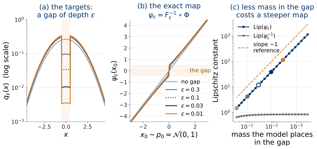
Take the line, the source \(p_0 = \mathcal{N}(0, 1)\), and a family of targets \(q_\varepsilon\) built as a Gaussian bulk of width \(1.5\) whose density is multiplied by \(\varepsilon\) on the gap \((-\tfrac12, \tfrac12)\). At \(\varepsilon = 1\) there is no gap; as \(\varepsilon \to 0\) the gap becomes a hard-zero gap, the one-dimensional checkerboard. For every \(\varepsilon > 0\) the target has support \(\mathbb{R}\), like the source, so the proposition does not apply: exact equality is possible, and the unique increasing map that achieves it is the quantile transform \(\psi_\varepsilon = F_\varepsilon^{-1} \circ \Phi\), with \(F_\varepsilon\) the target’s distribution function and \(\Phi\) the standard normal one. Its slope is the one-dimensional change of variables read backwards, \(\psi_\varepsilon'(z) = \varphi(z) / q_\varepsilon(\psi_\varepsilon(z))\): small target density means large slope. (Because \(q_\varepsilon\) jumps at the gap edges, \(\psi_\varepsilon\) is a homeomorphism with one-sided slopes at two points, not a diffeomorphism; nothing below needs more.) Figure 4 plots the family, the maps, and the constants.
scripts/python/fig_u1_t2_gap_bilipschitz.py.
Read panel (c) as Corollary 2.2 with the function \(M\) made explicit for one family: to leave a fraction \(m\) of the mass in the gap, the map must have a Lipschitz constant of order \(0.4 / m\). Halve the bridge, double the steepness. And the constant grows only in one direction — the inverse \(\psi_\varepsilon^{-1}\) stays bounded — because the price of a gap is paid where the map must stretch a sliver of source mass across a region the target barely covers. This is one dimension, one family, one exact map; it is not a theorem about \(d = 2\) or about trained models. It is what the theorem’s conclusion looks like when every quantity in it can be written down.
The animation below runs the family as a sweep instead of five snapshots: \(\varepsilon\) goes from \(1\) to \(0.01\), and three numbers run beside the map, computed at every frame: the mass in the gap, \(\operatorname{Lip}(\psi_\varepsilon)\) and \(\operatorname{Lip}(\psi_\varepsilon^{-1})\).
At \(\varepsilon = 1\) the target is \(\mathcal{N}(0, 1.5^{2})\) and the map is the straight line \(1.5\,x_0\), so the first reading, \(1.50\), is a slope everywhere and not yet a price. From \(\varepsilon \le 0.3\) on, the largest slope sits at the edge of the gap (the orange dot), and it climbs to \(12.1\) at \(\varepsilon = 0.1\) and to \(118\) at \(\varepsilon = 0.01\), while the inverse never passes \(0.850\). The last frame draws the limit \(\varepsilon = 0\) dashed, as a separate object and not as a frame of the sweep: the map jumps from \(-\tfrac12\) to \(+\tfrac12\) at \(x_0 = 0\), it is no longer a homeomorphism, and §5, the support proposition takes over.
Reading the checkerboard correctly
Now Table 1 can be read. Every finite, regular, Gaussian-based flow assigns nonzero density to the gaps: structural, by Equation 11. But the amount of bridge mass is not fixed by topology. It can be pushed toward zero, at the cost of increasingly extreme distortion, by Cornish’s theorem and by Figure 4. So \(29.8\%\) is a number about one six-layer model trained for 8000 steps at a bounded log-scale, not a number about diffeomorphisms. A deeper model, or one whose scale bound is relaxed, could put less mass in the gaps, and would pay for it in conditioning. The half nat above \(\log 18\) is the same story: no flow of this unit reaches \(\log 18\) exactly, but there is no positive floor either — the excess is \(\mathrm{KL}(q \,\Vert\, p_\theta)\), which a model with mass \(1 - \delta\) on the squares brings down to \(-\log(1 - \delta)\), arbitrarily close to zero at the conditioning cost of §5, Cornish’s strengthening. The \(0.50\) is what this architecture paid.
| Observation on a trained flow | Status |
|---|---|
| nonzero model density in hard-zero gaps | structural under a full-support source and a diffeomorphism (Equation 11) |
| increasingly extreme Jacobian or log-scale conditioning as the mismatch is pushed harder | supported by the topology/conditioning theorem (Equation 13) |
| inverse round-trip degradation, numerical instability | plausible numerical consequence of a large bi-Lipschitz constant; measure it |
| NLL plateau, poor samples | non-specific: capacity, optimization, or the learning rate can each produce it |
Where the obstruction goes next
- U2. A flow defined by a well-posed ordinary differential equation is still a diffeomorphism of \(\mathbb{R}^{d}\) onto itself. Continuous time changes the parameterization and the cost structure of the map; it does not remove a constraint that holds for every homeomorphism. U2 adds a separate, continuous-time restriction of its own; the two are kept apart on purpose, and U3 recalls both.
- U3. A target with an exact hard support forces a choice at the data end of the path from \(p_0\) to \(q\): a singular or limiting endpoint, or a deliberately smoothed one. U3 revisits this when it designs that path.
- U6, manifolds. When the data space itself has a non-Euclidean topology, the fix is not a better flow on \(\mathbb{R}^{d}\) but a source and a map that live on the right space; and a regular flow on that space is still a diffeomorphism of it, so the proposition of §5, the support proposition applies there unchanged.
topology-obstruction-argument is consumed as a whole — proposition, strengthening, diagnostics — by U2.T1, U3.T1, the U6 speaker kit and the U7 workshops. Its semantics are fixed here: supports and conditioning, never density level sets. A later session that quotes it the other way is misquoting it.
§6 — Residual flows: invertibility without triangularity
Reference for this section: (Behrmann et al. 2019) §2–3 (invertible residual networks) and (Chen et al. 2019) (residual flows), with (Papamakarios et al. 2021) §3.3.1 as the survey account. This section produces the artifact hutchinson-estimator. Everything so far bought a cheap log-determinant by forcing the Jacobian to be triangular. Residual flows give that up, take a dense Jacobian, and pay for it differently.
The dialect, declared once
Residual-flow papers write the map in the direction a residual network computes it, from the data to the source. That is the density transform, and in course notation it is \[ f = \psi^{-1}, \qquad f(x) = x + g(x), \tag{14}\]
with \(g \colon \mathbb{R}^{d} \to \mathbb{R}^{d}\) a network — the residual branch of an ordinary residual block. A flow is a stack of such blocks. The course convention \(\psi \colon z \to x\) stands; \(f\) is the letter this page uses for \(\psi^{-1}\), as U1.T1’s library-dialect note allowed.
Why this could be invertible at all. A residual block is the identity plus a perturbation. If the perturbation is small enough in the right sense, the identity wins and the map is a bijection. “Small enough” is a Lipschitz condition.
Invertibility by Banach
Fix \(z\) and ask for \(x\) with \(x + g(x) = z\). Rearranged, that is a fixed-point equation, \(x = z - g(x)\), and the natural iteration is \[ x^{(m+1)} = z - g\big(x^{(m)}\big), \qquad x^{(0)} = z . \tag{15}\]
Let \(\operatorname{Lip}(g) = L < 1\), that is, \(\lVert g(x) - g(x')\rVert \le L \lVert x - x'\rVert\) for all \(x, x'\). Then the map \(T_z(x) = z - g(x)\) is an \(L\)-contraction: \[ \lVert T_z(x) - T_z(x')\rVert = \lVert g(x') - g(x)\rVert \le L\,\lVert x - x'\rVert . \tag{16}\]
That is the whole live proof: two lines, and the second is the definition of \(L\). The rest is the Banach fixed-point theorem on the complete metric space \(\mathbb{R}^{d}\), which gives a unique fixed point \(x^{\ast}\) of \(T_z\), hence a unique solution of \(f(x) = z\) — so \(f\) is a bijection of \(\mathbb{R}^{d}\) onto \(\mathbb{R}^{d}\), and Equation 15 converges to its inverse from any starting point (Behrmann et al. 2019, Thm. 1). Completing the argument is PS1.5.
Let \(g \colon \mathbb{R}^{d} \to \mathbb{R}^{d}\) have \(\operatorname{Lip}(g) = L < 1\) and \(f(x) = x + g(x)\).
(a) Show that \(T_z(x) = z - g(x)\) is an \(L\)-contraction (Equation 16, written out with the definitions).
(b) Apply the Banach fixed-point theorem on \(\mathbb{R}^{d}\) — state why \(\mathbb{R}^{d}\) with the Euclidean norm is complete — to conclude that \(f\) is a bijection of \(\mathbb{R}^{d}\) onto \(\mathbb{R}^{d}\) and that Equation 15 converges to \(f^{-1}(z)\) from every \(x^{(0)}\).
(c) Show \(\operatorname{Lip}(f) \le 1 + L\) and \(\operatorname{Lip}(f^{-1}) \le 1 / (1 - L)\). Conclude that \(f\) is a homeomorphism, and, when \(g\) is \(C^{1}\), a diffeomorphism (the Jacobian \(I + J_g\) is invertible because \(\lVert J_g \rVert_2 \le L < 1\)).
(d) Bonus. Prove the a-priori bound \(\lVert x^{(m)} - x^{\ast}\rVert \le \dfrac{L^{m}}{1 - L}\, \lVert x^{(1)} - x^{(0)}\rVert\), and use it to give the number of iterations that guarantees a tolerance \(\delta\). State what this means for the cost of drawing one sample from a \(K\)-block residual flow.
Assigned today. Part (c) is the bound quoted in §5, Cornish’s strengthening; part (d) is the dashed line in Figure 5(a).
How the condition is enforced. \(g\) is a composition of \(1\)-Lipschitz nonlinearities and linear layers, and \(\operatorname{Lip}\) is submultiplicative, so it suffices to divide each weight matrix by a number larger than its spectral norm: spectral normalization (Behrmann et al. 2019, sec. 2.1). That is a constraint on the architecture, enforced throughout training, and it is exactly the bounded bi-Lipschitz constant that §5, Cornish’s strengthening turned into a limitation.
The log-determinant, as a series
The Jacobian of the block is \(J_f = I + J_g\), and it is dense: nothing here is triangular, and \(\det(I + J_g)\) has no closed form. Two facts hold under the Lipschitz condition. First, the determinant is positive: every eigenvalue \(\lambda\) of \(J_g\) has \(\lvert\lambda\rvert \le \lVert J_g \rVert_2 \le L < 1\), so every eigenvalue \(1 + \lambda\) of \(J_f\) has positive real part, and the product of them — real ones positive, complex ones in conjugate pairs — is positive (Behrmann et al. 2019, Lemma 6). Second, the logarithm of the determinant is the trace of the matrix logarithm, and the matrix logarithm has a power series.
\[ \begin{aligned} \log\det\big(I + J_g\big) &= \operatorname{tr}\log\big(I + J_g\big) \\ &= \sum_{k=1}^{\infty} \frac{(-1)^{k+1}}{k}\,\operatorname{tr}\big(J_g^{k}\big), \\ &\phantom{=}\ \text{valid when } \rho(J_g) < 1, \end{aligned} \tag{17}\]
where \(\rho\) is the spectral radius, and \(\rho(J_g) \le \lVert J_g\rVert_2 \le \operatorname{Lip}(g) < 1\) in the regime of this section.
The condition is part of the formula. This is the Maclaurin series of \(\log(1 + a)\) with a matrix in place of \(a\), and it converges for exactly the same reason and under exactly the analogous condition. Do not present it as formal algebra valid for any \(J_g\); for a block whose residual branch is not contractive the right-hand side diverges. Write \(\mathrm{PS}_n\) for the partial sum of the first \(n\) terms. The truncation error \(\lvert \mathrm{PS}_n - \log\det(I + J_g)\rvert\) is bounded by \(d \sum_{k > n} L^{k}/k\) (Behrmann et al. 2019, Thm. 3), geometric in \(n\) at rate \(L\) — fast for \(L = 0.5\), slow for \(L = 0.95\), as Figure 5(b) shows.
Hutchinson’s estimator
The series trades one dense determinant for infinitely many traces of matrix powers, and a trace of a \(d \times d\) matrix that is never formed is itself expensive: \(\operatorname{tr}(J_g)\) exactly costs \(d\) backward passes. The device that makes the series usable is an unbiased estimator of a trace from a random vector.
Let \(A \in \mathbb{R}^{d \times d}\) and let \(v\) be a random vector with \(\mathbb{E}_{v}[v v^{\top}] = I_d\) — Rademacher entries \(\pm 1\), or \(v \sim \mathcal{N}(0, I_d)\). Then \[ \operatorname{tr}(A) = \mathbb{E}_{v}\big[\, v^{\top} A\, v \,\big]. \tag{18}\]
Usage. \(v^{\top} J_g^{k} v\) is computed by \(k\) vector–Jacobian products, \(w^{\top} \leftarrow v^{\top}\), then \(w^{\top} \leftarrow w^{\top} J_g\) repeated \(k\) times, then \(w^{\top} v\); each product costs about one backward pass of \(g\), and \(J_g\) is never materialized. One probe \(v\) serves every term of the truncated series.
Deferred. The proof of Equation 18, and the analysis of the estimator’s variance, are written out in U2.T2, where the estimator becomes load-bearing for a continuous-time model. This page states it and uses it.
Two further points, both named and not developed. The estimator of Equation 18 is unbiased for each term of Equation 17, but a truncated series is biased; the Russian-roulette estimator of (Chen et al. 2019) removes that bias: it truncates at a random depth and reweights the terms that survive so that the expectation is the full sum. The name is enough today. And the estimate has variance, which one probe per data point does not remove; Figure 5(c) shows what that variance looks like on one matrix.
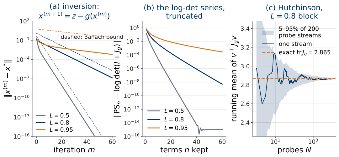
scripts/python/fig_u1_t2_resflow.py.
Residual flows on the table
| Density / likelihood | Sampling | |
|---|---|---|
| Residual flow | \(f(x) = x + g(x)\) is direct, one forward pass per block; \(\log\lvert\det J\rvert\) is an infinite series, estimated stochastically (Equation 17 with Equation 18, truncated or Russian-roulette) | \(\psi = f^{-1}\) by fixed-point iteration (Equation 15), several evaluations of \(g\) per block |
One row is stochastic and approximate, the other is iterative. Neither is analytic. Do not say that both directions are intrinsically stochastic: the sampling direction is exact to any tolerance, at the cost of iterations.
U2.T1 reuses the Lipschitz-and-uniqueness logic of §6, Banach for the flows of differential equations. U2.T2 reuses Equation 18 for a trace that is much simpler than Equation 17 — a single trace, not a series of them — and that is where the estimator’s proof is written and its variance measured.
§7 — Depth to infinity: the cliffhanger
Reference for this section: (Behrmann et al. 2019) §2, which opens with the observation below, and (Papamakarios et al. 2021) §3.3.1. This section gestures; it does not derive.
A residual stack with a step size
Write a residual stack with an explicit step size \(h > 0\) in front of each residual branch, and let the branch depend on a layer index turned into a time \(t_k = k h\): \[ \begin{aligned} &x_{k+1} = x_k + h\,f(t_k, x_k), \\ &k = 0, \dots, K - 1, \quad h = 1/K . \end{aligned} \tag{19}\]
The letter \(f\) changes its meaning here, deliberately: it is now the right-hand side of a differential equation, written time-first as the course’s code convention f(t, x) requires; the residual branch of §6 is \(g_k(x) = h f(t_k, x)\). Equation 19 is the forward-Euler discretization, with step \(h\), of \[
\frac{\mathrm{d}x}{\mathrm{d}t} = f(t, x), \qquad t \in [0, 1],
\tag{20}\]
and as \(h \to 0\) the stack’s output \(x_K\) converges to the solution \(x(1)\) of Equation 20 started at \(x_0\). Figure 6 measures it on one field.
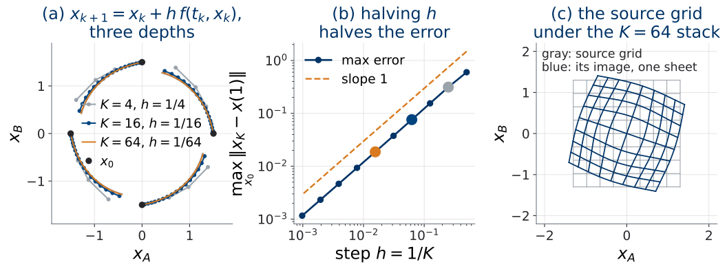
scripts/python/fig_u1_t2_euler.py.
Panel (c) is the bridge between §5, §6 and §7 in one picture. Each Euler block \(x \mapsto x + h f(t_k, x)\) has residual branch \(h f(t_k, \cdot)\) with Lipschitz constant \(h \operatorname{Lip}(f)\). The field was chosen to be Lipschitz on the whole plane — a cubic pull would not be, and then no step \(h\) would make the block a contraction perturbation everywhere — so once \(h < 1 / \operatorname{Lip}(f)\) each block satisfies §6’s contraction condition and the stack is a homeomorphism of \(\mathbb{R}^{2}\). By §5’s proposition its image of the grid is one connected sheet, which is what the panel shows. The qualifier “the field still needs regularity” of §7, the promise is this sentence.
The animation below follows panel (a) one doubling at a time, on the same four starting points. \(K\) goes from \(2\) to \(256\): every segment of the stack splits at its midpoint, and the new vertices move onto the stack with \(2K\) blocks. The gray curves stay fixed; the only thing that changes is \(K\).
For these four points the largest endpoint error falls from \(0.6014\) at \(K = 2\) to \(0.0047\) at \(K = 256\), and every ratio between consecutive doublings lies between \(1.91\) and \(2.03\): the drawn points show the same first-order rate as the cloud of panel (b). The last frame states the question that §7, the promise leaves open: the stack’s log-determinant is a sum of \(K\) terms, and what that sum becomes as \(K \to \infty\) is not derived here.
The promise, without overclaiming
What continuous time will and will not buy, stated now so that U2 can be held to it:
- Discrete residual invertibility (§6) needed a strong layerwise condition: every block a contraction. That is what bounded the bi-Lipschitz constant in §5, Cornish’s strengthening and what spectral normalization enforces.
- A well-posed differential equation Equation 20 is invertible on its interval under the usual existence-and-uniqueness and no-blow-up conditions: run it backwards. The vector field still needs regularity — a Lipschitz-type assumption on \(f\) does not disappear — but the architecture is no longer forced to make every finite residual block a contraction. The condition moves from the layers to the field.
- The log-determinant of the stack is a sum over \(K\) blocks of \(\log\det(I + h J_f)\). As \(h \to 0\) and \(K \to \infty\) that sum wants to become an integral. What it becomes is not derived here.
What does \(\log\lvert\det J\rvert\) become in continuous time?
Not answered today. U2.T1 sets up the flows of differential equations and the cost of running a solver inside every training step; U2.T2 answers this question, and §6’s trace estimator is on the answer’s critical path.
§8 — Unit close: the two costs, version 2
The persistent board of the live session is U1.T1’s table, filled row by row during §2, §3 and §6. Here it is as it stands at the end of the unit, with the same box name and one row per family.
| Family | Density / likelihood | Sampling | Main trick, and its price |
|---|---|---|---|
| NICE / RealNVP | exact: analytic inverse, triangular log-determinant | direct | coupling; depth and permutations |
| Glow | exact | direct | channel mixing and multi-scale engineering |
| MAF | fast, parallel density transform | sequential inverse, in the event dimension | autoregressive direction, data side |
| IAF | sequential inverse for density | fast, parallel generative map | autoregressive direction, source side |
| Residual flow | direct density map; log-determinant a stochastic series | iterative inverse | contraction condition and trace estimators |
Reading the unit. Exactness was achieved in U1.T1, by construction. The architecture choices of this page expose computational dualities: a triangular structure can be read in either direction, and the direction decides which cost is sequential (§3). Support topology and conditioning revealed a real limitation, not a capacity gap, and gave a calibrated way to tell the two apart (§5). Residual flows dropped triangularity, paid with a series and an iteration (§6), and pointed at continuous time as the escape from architectural bookkeeping — not from mathematics: the map is still a diffeomorphism, the field still needs regularity, and the log-determinant still has to be paid for, in a currency U2 names (§7).
§9 — Exercises, with answers
Work these before reading the answers. Each one is a claim made on this page in passing.
Exercise 1 — a level of Glow, by hand
A \(4 \times 4 \times 2\) tensor passes through one squeeze, one actnorm with \(s = (2, \tfrac12, 1, 4, 1, 1, \tfrac14, 2)\), and one \(1 \times 1\) convolution with \(W = PL(U + \operatorname{diag}(s'))\), \(s' = (1, 1, 3, \tfrac13, 1, 2, 1, \tfrac12)\). Give the total \(\log\lvert\det J\rvert\).
Squeeze is a reshape to \(2 \times 2 \times 8\): log-determinant \(0\), and \(h w = 4\) from here on. Actnorm contributes \(4 \sum_c \log\lvert s_c\rvert = 4 (\log 2 - \log 2 + 0 + \log 4 + 0 + 0 - \log 4 + \log 2) = 4 \log 2\). The convolution contributes \(4 \sum_i \log\lvert s'_i\rvert = 4(0 + 0 + \log 3 - \log 3 + 0 + \log 2 + 0 - \log 2) = 0\). Total: \(4 \log 2 \approx 2.77\). No determinant was computed, and \(P\), \(L\), \(U\) never entered.
Exercise 2 — the sequential direction, written out
For a MAF with \(d = 3\) and affine conditioners, write the recursion that computes \(x = \psi(z)\) from \(z\), and count how many times the conditioner network is evaluated if nothing is cached. Then do the same for the density direction of an IAF.
MAF, sampling: \(\xi_1 = \mu_1 + \sigma_1 \zeta_1\) (the first conditioner reads nothing); \(\xi_2 = \mu_2(\xi_1) + \sigma_2(\xi_1)\,\zeta_2\); \(\xi_3 = \mu_3(\xi_1, \xi_2) + \sigma_3(\xi_1, \xi_2)\,\zeta_3\). Each line needs the previous lines’ outputs, and with a single masked network that produces all \((\mu_i, \sigma_i)\) at once, the network is run three times, once per coordinate, with the input filled in progressively — \(d\) passes for \(d = 3\). IAF, density: \(\zeta_1 = (\xi_1 - \mu_1) / \sigma_1\); \(\zeta_2 = (\xi_2 - \mu_2(\zeta_1)) / \sigma_2(\zeta_1)\); \(\zeta_3 = (\xi_3 - \mu_3(\zeta_1, \zeta_2)) / \sigma_3(\zeta_1, \zeta_2)\): the same three passes, on the other side. This is the “\(d\) passes” intuition, and it is exact for this conditioner; a conditioner that caches its earlier outputs changes the count without changing the sequential dependence.
Exercise 3 — the scalar series, and its condition
For \(d = 1\) the block is \(f(x) = x + g(x)\) with \(g'(x) = a\) at the point of interest. Write Equation 17 in this case, say for which \(a\) it converges, and say what goes wrong at \(a = -1\) and at \(a = 1\).
\(\log(1 + a) = \sum_{k \ge 1} (-1)^{k+1} a^{k} / k\), the Maclaurin series, which converges exactly for \(-1 < a \le 1\). At \(a = -1\) the block has \(f'(x) = 0\): it is not locally invertible, the determinant is \(0\), its logarithm is \(-\infty\), and the series diverges to \(-\infty\) as it should. At \(a = 1\) the series converges (to \(\log 2\)) but only conditionally, and for any \(a > 1\) it diverges although \(\log(1 + a)\) is perfectly finite. That last case is the point: the series is not the log-determinant unless the condition holds. The contraction hypothesis \(\lvert a\rvert \le L < 1\) keeps every block strictly inside the disk of convergence, with a geometric tail.
Exercise 4 — an Euler block is a residual-flow block
Let \(f(t, \cdot)\) be \(\Lambda\)-Lipschitz on \(\mathbb{R}^{d}\) for every \(t\). Show that the map \(x \mapsto x + h f(t, x)\) is a bijection of \(\mathbb{R}^{d}\) onto itself whenever \(h \Lambda < 1\), and give the iteration that inverts it.
Put \(g(x) = h f(t, x)\). Then \(\lVert g(x) - g(x')\rVert = h \lVert f(t, x) - f(t, x')\rVert \le h \Lambda \lVert x - x'\rVert\), so \(\operatorname{Lip}(g) \le h \Lambda < 1\) and §6, Banach applies verbatim: the map \(x + g(x)\) is a bijection of \(\mathbb{R}^{d}\) onto itself, and \(x^{(m+1)} = y - h f(t, x^{(m)})\) converges to its inverse at \(y\) from any starting point, at rate \(h \Lambda\). This is how Figure 6(c) was inverted, block by block, backwards through the stack: \(64\) blocks with \(h \Lambda \le 0.041\), round trip \(1.2 \times 10^{-15}\). The hypothesis is global: \(\Lambda\) must bound the Lipschitz constant on all of \(\mathbb{R}^{d}\), which is why the figure’s field has a damped pull.
Reading the board
The live session closes by reading its board. Here is the same reading.
| On the board | Status |
|---|---|
| The depth question — how expressive is a stack of coupling layers? | Answered, twice. Volume-preserving stacks are not universal, and keep the base’s mode count (§4, volume-preserving). Affine coupling stacks are universal for continuous targets of infinite support, in the sense and with the fine print of §4, affine coupling and the fine print. |
| The fine print — a flow is a diffeomorphism | Examined. A homeomorphism of \(\mathbb{R}^{d}\) preserves the support’s topology (§5, the support proposition), so a flow of this unit has support \(\mathbb{R}^{d}\) and cannot equal a disconnected or lower-dimensional target; approaching one costs conditioning without bound (§5, Cornish’s strengthening). Not a statement about level sets (§5, level sets). |
| The checkerboard gaps | Explained, and calibrated. Nonzero gap density is structural; the amount is this model’s, not a theorem’s (§5, reading the checkerboard, Table 2). |
| The two costs | Version 2 (Table 3): five families placed. |
| New — what does \(\log\lvert\det J\rvert\) become in continuous time? | Open. U2. |
Where this page reappears
| From this page | Reappears in |
|---|---|
| Glow’s layers, §2 | U1.L2 (the multi-scale stack, executable) |
| The task-direction table, Section 3.4 | every library cross-check of the course |
| Universality with its fine print, §4 | U3.T1 (kept distinct from topology and from conditioning when the path’s endpoint is chosen) |
topology-obstruction-argument, §5 |
U2.T1 (kept separate from the continuous-time restriction); U3.T1; U6 speaker kit; U7.W1 (Table 2 as a debugging aid); U7.W2 |
| The one-dimensional gap family, Figure 4 | U3, when the data end of the path is designed |
| Banach invertibility, §6 | U2.T1 (existence and uniqueness for flows of differential equations); PS1.5 |
hutchinson-estimator, Equation 18 |
U2.T2 (v2: proof and variance, in place); U2.L2 |
| The Euler rewrite, Equation 19 | U2.T1, first slide |
two-costs-table v2, Table 3 |
U2.T2 (v3); U3.L1 |
Next session
The next session is the lab (U1.L2): multi-scale flows on images, where the squeeze-and-split bookkeeping of Figure 2 becomes code and a bits-per-dimension protocol is fixed for the rest of the course. The theory session after it opens U2 on the question left on the board.
Before then: PS1.5 (Section 6.2) is assigned today.