U2.L1 — Solvers and Adjoints in Practice

Session U2.L1 · date: see calendar-map

How to read this page. The previous session (U2.T1) proved the adjoint theorem and wrote a table with three columns: memory, compute, correctness. Every cell of that table was an argument. Today every cell becomes a measurement. The object is a small Neural ODE that classifies the two-moons points, a task on which nothing hurts yet; that is deliberate. You learn the instruments here, on a problem where nothing is at stake, so that the next lab (U2.L2) can point them at a generative model and the readings there say something about the problem, not about unfamiliar tooling.

These notes are the written record of the lab; the executable part is the notebook labs/lab-u2l1.ipynb; the instructor releases its solutions, lab-u2l1-solutions.ipynb. The page is self-contained on purpose. It depends on two sessions, U2.T1 and U1.L1, and on the solver notes of U0.T5 (also in the self-study packet), which the entry quiz checks. Where a bootcamp artifact is named, its contract is written out here in full, and you do not need to have attended the bootcamp.

Every number on this page was measured. The runs are in scripts/python/fig_u2_l1_instruments.py, seeded, with torch on one thread of an Intel Core Ultra 9 185H CPU (JAX uses its own thread pool; the memory figure alone uses a GPU, and says which). The values are recorded in scripts/python/_outputs/u2l1_instruments.json. Counts, errors and gradients reproduce to the digit on a re-run. Wall-clock times do not, and every time on this page is on the machine named here, unless the text names another; GPU memory peaks move by up to 20 KiB between repetitions (the recorded spread), and the CPU memory readings are coarse: recorded once, and asserted on nothing.

The libraries are torchdiffeq (Chen 2018) and Diffrax (Kidger 2021); their READMEs are linked from the notebook header. The adjoint is the one of Chen et al. (2018, sec. 2), derived in U2.T1 after Massaroli et al. (2020, App. A.1).

The instrument panel you leave with

An NFE counter: three lines that count every call of the field.
NFE-against-quality axes: what a solver setting buys, on two metrics that do not agree.
NFE drift in training: the cost of one forward solve, logged at every optimizer step.
A peak-memory protocol: the GPU allocator’s peak, reset and synchronized around one forward-and-backward pass.
A gradient-fidelity table: two differentiation routes against a finite difference that owes nothing to either.
Honest timing: compile time reported apart from steady state.

Nothing on this page is about generative models. The classifier is the point: the instruments have to be trusted before the reading matters.

0 · Orientation, and the entry quiz

Block 0, 10 minutes.

Given code

Table 1: The given code, and where it came from. Provenance is not a prerequisite.

Module	Built in	What this lab uses
`common/toy2d.py`	U1.L1 (frozen)	`two_moons(n, seed)`, a `(n, 2)` float32 tensor
`common/odesolve.py`	U0.L5 (frozen)	`odeint(f, x0, t0, t1, method="rk4", n_steps=N)`, whose result carries `.nfe`
`common/train.py`	U0.L1, extended in U0.L2	`set_seed(seed)` only

Two moons as a classification task. U1.L1 froze two_moons as a sampler with no labels. Its contract fixes the order of the rows: the first n // 2 points lie on the upper moon and the rest on the lower moon. So the label is the row order, and the frozen file does not change:

x = two_moons(n, seed)
y = (torch.arange(n) >= n // 2).long()      # 0 = upper moon, 1 = lower moon

The script checks that this reading is right: the mean second coordinate is 0.85 for label 0 and −0.97 for label 1. The training set is two_moons(512, 0), the test set two_moons(2048, 1).

The training loop is written out, not the given Trainer. The reason is an instrument: the NFE counter must be read between the forward solve and the backward pass of every step, and the Trainer has no hook there. The loop is about a dozen lines (§1); the seeding, the optimizer schedule and the logging conventions of the course hold, with one logging departure named below.

Where the numbers go

The course logs to MLflow, deployed locally: a SQLite file next to the notebook (sqlite:///mlflow.db) and a mlartifacts/ directory. This lab uses the experiment U2, one run per block, tagged session=U2.L1 and block=<n>, with the resolved configuration as parameters. One departure, with its reason: the loop measures the wall-clock of every step (a median of 53 ms here), and a SQLite write inside the loop would become part of what it measures. So the curves are logged after the loop, in one batch, from the lists the loop kept. The run stands alone either way.

The entry quiz

This lab assumes, without teaching it again, what the solver notes of U0.T5 (also in the self-study packet) say about adaptive solvers (U0.T5, Adaptive stepping and Stability). Six questions check it. Answer them on paper before you open the answers (at the end of this page). With four or more right, go on. With fewer, read those two sections of U0.T5 before §2; §1 does not need them.

What does NFE count, and why does the course report it for every solve?
An adaptive solver takes rtol and atol. Where does each one dominate?
Why does an adaptive solver reject a step, and what does a rejected step cost?
What is dopri5?
For a fixed-step method, what decides the cost of a solve? For an adaptive one?
What does it mean, loosely, for an equation to be stiff?

1 · A Neural ODE classifier on two moons

Block 1, 20 minutes.

The model, and why its state stays in the plane

The model is U2.T1’s Neural ODE (U2.T1, The model), used as a feature map. An input point \(x_0 \in \mathbb{R}^2\) is the initial state; the flow carries it to \(x(1) = \psi_1(x_0)\); a linear head reads the class from the endpoint. Here \(x_0\) is an input point, not a sample of the source distribution: a classifier’s flow has no generative direction, and the course’s time arrow (noise at \(t = 0\), data at \(t = 1\)) does not apply to it.

\[ \begin{aligned} \dot x(t) &= f_\theta\big(t, x(t)\big),\quad x(0) = x_0,\quad t \in [0, 1],\\ \text{logits} &= W\,\psi_1(x_0) + b,\quad W \in \mathbb{R}^{2\times 2}. \end{aligned} \]

The field is a small network with the time supplied as an input, \(f_\theta(t, x) = W_3 \tanh\big(W_2 \tanh(W_1 [x; t] + b_1) + b_2\big) + b_3\), with two hidden layers of width 32. With the head, the model has 1,256 parameters. Two choices in it are deliberate.

The state stays in the plane. The ODE runs in \(\mathbb{R}^2\), where the data live, so a picture of the trajectories is a picture of the actual state. A model whose state lives in \(\mathbb{R}^8\) would need a projection to be drawn, and a projection of eight-dimensional curves onto a plane can show crossings that do not exist in the state. The checkpoint below makes a claim about the state, so the state must be what is drawn.

The activation is smooth. \(\tanh\) is \(C^\infty\) with \(\lvert \tanh' \rvert \le 1\), so \(f_\theta\) is continuously differentiable in \((t, x, \theta)\) and globally Lipschitz in \(x\), uniformly in \(t\), with a constant at most \(\lVert W_3 \rVert \, \lVert W_2 \rVert \, \lVert W_1 \rVert\) (operator norms). Those are both tiers of U2.T1’s regularity contract (U2.T1, The standing regularity contract); Tier 2 is what the adjoint theorem assumes.

The loss is the cross-entropy of the head’s prediction, averaged over the training set, with the sampling written out:

\[ \ell(\theta) = \mathbb{E}_{(x_0, y) \sim \mathcal{D}_{\mathrm{train}}} \Big[ -\log \operatorname{softmax}\big(W\,\psi_1(x_0) + b\big)_{y} \Big], \]

where \(\mathcal{D}_{\mathrm{train}}\) is the empirical distribution of the 512 labelled training points and \(\theta\) collects the field’s parameters and \((W, b)\). Each term is U2.T1’s terminal loss \(L_y\big(x(1)\big)\), with \(L_y\) the head followed by the cross-entropy against the label \(y\), and \(\ell\) is their mean over \(\mathcal{D}_{\mathrm{train}}\). The head’s parameters enter only through \(L_y\), so their gradient needs no backward solve.

How much work does the flow do? The head alone, trained on the raw inputs with AdamW at \(3 \times 10^{-3}\) and weight decay 0.01 for 2000 full-batch steps, without a schedule, reaches 89.4% test accuracy: no line separates the two moons. Everything above that is the flow’s.

TODO 1.1 — the NFE counter

The number of function evaluations is the cost currency of this course: every solve reports it, and every later comparison is priced in it. You build the gauge yourself, once. It is a wrapper around the field:

class NFECounter(nn.Module):
    def __init__(self, f):
        super().__init__()
        self.f = f
        self.nfe = 0                     # 1
    def forward(self, t, x):
        self.nfe += 1                    # 2
        return self.f(t, x)              # 3

Two properties matter. It is an nn.Module that holds the field, so the field’s parameters are its parameters, and odeint_adjoint finds them without an adjoint_params argument in the adjoint runs of §3. And it counts every call, whoever makes it: the solver’s stages, its start-up calls, and, later, the calls the adjoint’s backward solve makes. Reset nfe to zero before a solve and read it after. Checkpoint 1.1 checks the count against arithmetic that the solver cannot fake: fixed-step Euler with \(N\) steps must report \(N\), and torchdiffeq’s rk4 must report \(4N\).

TODO 1.2 — train with the solver’s defaults

for step in range(300):
    t0 = time.perf_counter()
    model.field.nfe = 0
    logits = model(x, method="dopri5")      # rtol=1e-7, atol=1e-9: defaults
    nfe_fwd = model.field.nfe
    loss = F.cross_entropy(logits, y)
    opt.zero_grad(set_to_none=True)
    loss.backward()                         # direct backprop through dopri5
    opt.step(); sched.step()
    acc = float((logits.argmax(1) == y).float().mean())
    history.append((float(loss.detach()), acc, nfe_fwd,
                    model.field.nfe - nfe_fwd,        # backward calls
                    time.perf_counter() - t0))        # seconds

Five numbers per step: the loss, the training accuracy, the forward NFE, the backward NFE, and the seconds the step took. The solver is torchdiffeq’s dopri5 at its defaults, rtol \(= 10^{-7}\) and atol \(= 10^{-9}\). The optimizer is the U0.T2 recipe card (U0.T2, The recipe card): AdamW, weight decay 0.01, linear warmup over 3% of the steps and then cosine decay, stepped per step, full batch (512 points). One deviation, in writing, with its reason. The base learning rate is \(3 \times 10^{-3}\), not the card’s \(3 \times 10^{-4}\). At the card’s rate, the same model and seed trained for 1500 steps (five times as many, 77 s) end at a training loss of 0.0275 and 99.6% training accuracy; at step 300 of that run the loss is still 0.287. At \(3 \times 10^{-3}\), 300 steps take 15.1 s and end at 0.0032, 8.5 times lower. Five times the steps do not close the gap, and the block has other work to do in its twenty minutes.

The reference run ends at 100.0% test accuracy and a test cross-entropy of 0.0029. One forward solve of the test set at the defaults costs 116 evaluations. And the backward pass calls the field zero times, at every step: direct backprop replays the recorded operations, it does not evaluate \(f_\theta\) again. Keep that zero in mind for §3.

Why the head starts at zero

Card item 3 says: zero-initialize the last layer where “output \(\approx 0\) at start” is sensible. This model has two last layers, and both qualify. The field’s output layer starts at zero, so the flow starts at the identity. The head starts at zero, so the first prediction is uniform and the first loss is exactly \(\log 2 \approx 0.693\).

The second choice was not obvious in advance, and it was measured. With PyTorch’s default initialization of the head, seeds 2 and 3 of five stalled at every learning rate tried (\(3 \times 10^{-3}\) for 300 steps, \(10^{-3}\) for 600, \(3 \times 10^{-4}\) for 1500): their final training loss stayed at 0.23 or above, where every other run ended at 0.048 or below. The decision reads the training loss only; for the record, those runs reached test accuracies between 56.9% and 89.3%. With the head at zero, all 10 seeds tried reach 100.0% test accuracy, at \(3 \times 10^{-3}\) for 300 steps. A random head fixes a separating direction before the flow has learned anything, and a flow of the plane cannot move points through each other to repair a bad start. That sentence is an explanation of the measurement, not a theorem, and the page does not use it as one.

Zeroing both layers has one cost worth naming. At initialization the gradient of every field parameter is exactly zero, because it reaches the field through \(W = 0\). So the first update with a nonzero rate (step 2; step 1 has rate zero, from the warmup) changes the head, and the field’s output stays exactly zero, because its last layer is still zero. A gradient check run at initialization would measure nothing. No check on this page runs there: the fidelity checks of §3 use the trained model.

Checkpoint 1 — the trajectories in the plane

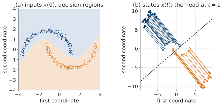
Figure 1: The reference model on the test set. (a) Every fifth test input \(x(0)\), and the decision regions, obtained by solving from every point of a \(161 \times 161\) grid. (b) Forty trajectories \(x(t)\), \(t \in [0, 1]\), twenty per class, in the actual state space: hollow markers at \(t = 0\), filled at \(t = 1\), and the head’s decision line at \(t = 1\) dashed. The flow moves the two classes apart until a line separates them.

Under the uniqueness assumptions of U2.T1 (Picard–Lindelöf), two distinct trajectories never occupy the same state at the same time. That is a theorem you already have; here it becomes a reading, with a stated floor. Over all 2,096,128 pairs of test points and 41 times, the ratio \(\lvert x^{(i)}(t) - x^{(j)}(t)\rvert / \lvert x^{(i)}(0) - x^{(j)}(0)\rvert\) stayed between 0.41 and 21.4: no pair closed to less than 0.41 of its starting separation. The script asserts a floor of 0.1, which a bug in the field or the solver could break; the measured floor is 0.41.

Read panel (b) with one caution. The field depends on \(t\), so two paths drawn in the plane may cross: a crossing of paths is two trajectories at the same place at different times, and uniqueness says nothing against it. None of the 40 drawn paths cross (0 crossings, counted by the script). If yours do, that is not a contradiction.

Optional warmup — your RK4 against the library’s

The first thing to skip when time is short. Integrate the trained field with the bootcamp’s own solver, common/odesolve.py, on a fixed grid, and compare the endpoints with a tight library reference (dopri5, rtol \(= 10^{-12}\), atol \(= 10^{-14}\), float64).

Table 2: Largest coordinate difference of the endpoints over the 2048 test points. From \(N = 16\) on, doubling \(N\) divides both errors against the reference by 14.0 to 15.5, near the \(2^4 = 16\) of order 4.

\(N\)	NFE	`odesolve` RK4 vs reference	torchdiffeq `rk4` vs reference	the two RK4s
8	32	\(5.4 \times 10^{-3}\)	\(5.0 \times 10^{-3}\)	\(3.4 \times 10^{-4}\)
16	64	\(4.3 \times 10^{-4}\)	\(4.1 \times 10^{-4}\)	\(2.5 \times 10^{-5}\)
32	128	\(3.1 \times 10^{-5}\)	\(2.9 \times 10^{-5}\)	\(1.6 \times 10^{-6}\)
64	256	\(2.1 \times 10^{-6}\)	\(2.0 \times 10^{-6}\)	\(9.9 \times 10^{-8}\)
128	512	\(1.3 \times 10^{-7}\)	\(1.3 \times 10^{-7}\)	\(6.2 \times 10^{-9}\)

The last column is not zero, and it should not be. torchdiffeq’s rk4 is the 3/8-rule fourth-order method, not the classical tableau of U0.T5 that odesolve implements. Both are order 4, both cost four evaluations per step, and on the same grid they are two different computations. The notebook’s threshold is calibrated on the reference run, not typed: at \(N = 64\) the measured error is \(2.1 \times 10^{-6}\), and the checkpoint asks for less than \(1 \times 10^{-4}\).

2 · Solver and tolerance sweep: NFE as the cost currency

Block 2, 20 minutes. The sweep (TODOs 2.1 and 2.2) is evaluation only: the model of §1 is fixed. TODO 2.3 re-trains a second seed for 100 steps.

TODO 2.1 — the sweep

Three families of solver settings, on the fixed checkpoint:

euler and rk4 with \(N \in \{4, 8, 16, 32\}\) fixed steps;
dopri5 with rtol \(\in \{10^{-1}, \dots, 10^{-7}\}\) and atol \(=\) rtol\(\,\times 10^{-2}\).

For each setting, record the NFE, the test accuracy, and the error of the terminal state against the tight reference of §1. The sweep runs in float64: this is a measurement, and the course rule is to train in float32 and promote the check. In float32, the tightest settings would measure round-off, not the solver.

The task metric may saturate before the trajectory error does. If it does, tighter tolerances spend evaluations without changing the classifier’s answer, and the choice of solver setting depends on which quantity you need to be right.

TODO 2.2 — two axes that disagree

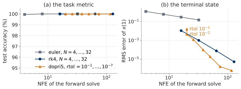
Figure 2: Fifteen solver settings on the fixed checkpoint, test set, float64. (a) Test accuracy against the NFE of one forward solve. (b) The RMS distance of the terminal state \(x(1)\) from the reference, against the same NFE. Both NFE axes are logarithmic, and so is the error axis of (b).

The hypothesis survives, in its strongest form. Test accuracy is 100% for 14 of the 15 settings; the exception is Euler with four steps, at 99.95% (1 point of 2048). Over the same settings the terminal-state error runs from 1.18 down to \(6.1 \times 10^{-7}\), more than 6 orders of magnitude. On this task accuracy is a nearly blind gauge for solver error. Euler with four steps has endpoints off by 1.18 in RMS and by 3.34 at worst, and it misclassifies 1 point of 2048: for every other point, the error does not carry the endpoint across the head’s line.

Panel (b) is the ancestor of every quality-against-cost plot in the rest of the course. Read one comparison off it, at similar cost: rk4 with 16 steps spends 64 evaluations and reaches \(7.5 \times 10^{-5}\), while dopri5 at rtol \(= 10^{-6}\) spends 74 and reaches \(1.6 \times 10^{-6}\): a fifth-order adaptive method against a fixed-step fourth-order one, so the comparison does not isolate the order. At the loosest tolerances the advantage is gone: dopri5 at rtol \(= 10^{-2}\) spends 20 evaluations for an error of \(4.4 \times 10^{-3}\), about the same as rk4 in the same range of cost.

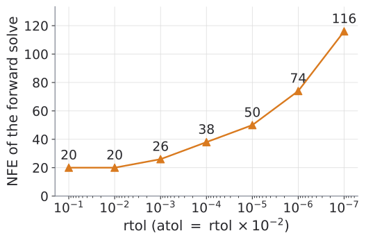
Figure 3: The NFE that `dopri5` spends on one forward solve of the test set, against the tolerance. At `rtol` \(= 10^{-1}\) and \(10^{-2}\) the cost is the same; tightening from \(10^{-6}\) to \(10^{-7}\) costs 42 more evaluations.

The curve of Figure 3 is data, not a law. A straight-line fit of \(\log \mathrm{NFE}\) against \(\log\) rtol over the five settings with rtol \(\le 10^{-3}\) has slope −0.16; that number describes this model at this checkpoint and predicts nothing about the next one.

One step size for the whole batch

U0.L5 made a point about batched adaptive solves: the error estimate is a tensor with the shape of the whole batch, and the controller reduces it to one number. torchdiffeq’s reduction is a root mean square over every element of the state. Measured on the reference model at the defaults: the batch of 2048 test points costs 116 evaluations, while 64 of those points, spread over both moons and solved one at a time, cost between 50 and 134 (median 74).

Two readings follow, and both matter for U2.L2. 60 of the 64 points pay more inside the batch than alone. And the hardest point gets fewer evaluations inside the batch (116) than it asks for alone (134): the tolerance holds for the batch’s RMS error, not for each point. U0.L5 put it as “one step size serves the hardest sample in the batch”. Under an RMS norm that is not so, and this measurement is the correction; a max norm would serve the hardest sample. The NFE of a batched adaptive solve is a property of the batch, and a change of batch composition changes it.

TODO 2.3 — NFE across training

A solver setting fixes a tolerance, not a cost. The cost depends on the field, and the field changes at every optimizer step. TODO 2.3 re-trains from a fresh initialization with a second seed, logs the primal (forward) NFE of each of the first 100 steps of the same schedule, and asks you to describe what happened. Nothing in advance says what you will see.

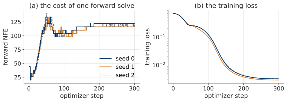
Figure 4: (a) The forward NFE of every training step, and (b) the training loss on a log scale, for the reference run and two more seeds, `dopri5` at its defaults; seed 2 is dashed, and in (b) its curve lies under seed 0’s. Three runs of one model on one task.

What happened in these three runs:

Steps 1 to 3 cost 44 each, for an arithmetic reason. The field is exactly zero for three solves: step 1 has learning rate zero (the warmup starts at zero), and at step 2 the field’s gradient is still exactly zero, because it reaches the field through \(W = 0\): the head learns, weight decay only shrinks the field’s hidden layers, and the field’s last layer stays zero (see Why the head starts at zero). With a zero field, torchdiffeq’s initial-step rule falls back to \(h = 10^{-6}\); every error estimate is then exactly zero, so the controller multiplies the step by its maximum factor, 10 in torchdiffeq (U0.T5’s controller uses 5). Seven steps cover \([0, 1]\): two start-up calls plus six new calls per dopri5 step, \(2 + 6 \times 7 = 44\). The script checks this count.
Then the cost falls, and rises. At step 4, the first solve of a nonzero field, the forward NFE drops to 20 (seed 0). It then climbs, to a peak of 134, 134 and 140 for the three seeds, reached at steps 48, 54 and 50. Over the same steps the loss drops from \(\log 2\) to 0.26, 0.25 and 0.26. After the peak the cost falls again, to 110, 104 and 104 at step 100, where TODO 2.3’s window ends, and then rises to its final level. Over the last 100 steps the NFE stays at 122 (seed 0) and 116 (seed 1), and moves between 116 and 122 (seed 2), while the loss goes on falling (panel (b) uses a log scale).
The seeds agree closely. Only the field’s hidden layers are random; both last layers start at zero in every seed.

That is a description of three runs, not a result about Neural ODEs. The same forward solve cost 20 evaluations at step 4 and 122 at step 300 (seed 0), with the solver settings unchanged. In U2.L2 you point this instrument at a generative model and read it again.

3 · Memory and gradient fidelity

Block 3, 20 minutes. The empirical companion to U2.T1’s table of the two gradient strategies (U2.T1, §5).

The method under measurement is Box U2.T1-3, the adjoint sensitivity theorem (U2.T1, The derivation), as torchdiffeq implements it in odeint_adjoint. The comparison is direct backprop through the solver, odeint. Both use fixed-step rk4, so the forward work is the same for both and only the backward pass differs.

The protocol

torch.cuda.synchronize(); torch.cuda.empty_cache()
torch.cuda.reset_peak_memory_stats()
base = torch.cuda.memory_allocated()     # model + data, already resident
loss = F.cross_entropy(model(x, adjoint=adj, method="rk4",
                             options={"step_size": 1 / N}), y)
loss.backward()
torch.cuda.synchronize()
peak = torch.cuda.max_memory_allocated() - base

The GPU allocator’s peak counter is the canonical meter, because every tensor the backward pass holds is allocated through it. Reset it and synchronize around each run, or the peak of an earlier run leaks into the next reading.

tracemalloc is not a meter for this. It traces allocations made through Python’s own allocator, and PyTorch allocates tensor storage in native code that tracemalloc does not see. It reports a number, and the number is not the memory the tensors occupy.

On a machine without a GPU, the notebook falls back to sampling the process’s resident set size (RSS) every millisecond. That reading is coarse and not a contract: the allocator reuses memory the process already holds, so a run can peak without the RSS moving. TODO 3.1 shows by how much.

TODO 3.1 — peak memory against the number of steps

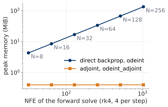
Figure 5: Peak GPU memory of one forward-and-backward pass (batch 512, float32) against the NFE of the forward solve, fixed-step `rk4` with \(N = 8, \dots, 256\) steps, on an NVIDIA GeForce RTX 4070 Laptop GPU. Direct backprop stores the solver’s work; the continuous adjoint does not.

Compare Figure 5 with U2.T1’s schematic (U2.T1, The plot you will make); it is the same picture, with numbers. Direct backprop grows from 4.33 MiB at \(N = 8\) to 134.26 MiB at \(N = 256\), a factor of 31 for a factor of 32 in steps: about 134 KiB per evaluation at this batch size. The adjoint holds 0.40 MiB at every \(N\). That is U2.T1’s claim at its stated strength: constant in the number of solver steps, for a fixed set of output times, not constant in everything.

The memory is not free, and the NFE counter shows the bill. On this fixed grid the adjoint’s backward pass calls the field exactly as many times as the forward pass did (\(N = 256\): 1024 calls forward, 1024 backward), because odeint_adjoint reuses the forward’s method and step size; an adaptive backward solve would choose its own steps. Each call adds vector–Jacobian products; direct backprop calls the field zero times. On this GPU the adjoint’s forward-plus-backward took 1.9 times as long as direct backprop at \(N = 8\) and 1.6 times at \(N = 256\) (one machine, median of three repetitions, descriptive).

The CPU fallback, measured. On the same configurations, the RSS reading for direct backprop was 127.8 MiB at \(N = 256\) against 134.26 on the GPU, and the trend is visible from \(N = 32\) up. The small runs are not: \(N = 8\) read 3.1 MiB against 4.33, and \(N = 16\) read 0.0 MiB against 8.52. The adjoint read 0.2 MiB at \(N = 8\), its first run, and 0.0 MiB at every larger \(N\). The allocator reuses memory the process already holds. That is what “coarse” means.

TODO 3.2 — the gradient-fidelity table

The course ritual (U0.L1): float64, one fixed unit direction \(v\), and a central difference as the witness that owes nothing to automatic differentiation. Here \(v\) is drawn over the parameters of \(f_\theta\) only, written \(\theta_f\) (\(v\) is zero on the head’s parameters): all three routes computed on the \(N\)-step grid pass through the head from the same endpoint, so the head’s term would be the same in each of them and would only dilute the gaps. Fix a batch \(B\) of 256 test points, and write the loss of the exact flow on it, and the loss as the computer evaluates it: \[ \ell_B(\theta) = \mathbb{E}_{(x_0, y) \sim B} \Big[ -\log \operatorname{softmax}\big(W\,\psi_1(x_0) + b\big)_{y} \Big], \] with the expectation uniform over the batch, and \(\ell_N\) the same with \(\psi_1\) replaced by \(N\) steps of rk4. Four directional derivatives:

\[ \begin{aligned} d_{\mathrm{FD}} &= \frac{\ell_N(\theta + \varepsilon v) - \ell_N(\theta - \varepsilon v)}{2\varepsilon},\\ d_{\mathrm{AD}} &= v^{\top} \nabla_{\theta_f} \ell_N \ \text{(direct backprop)},\\ d_{\mathrm{ADJ}} &= v^{\top} \hat g_N \ \text{(adjoint)},\\ d_{\mathrm{cont}} &= v^{\top} \nabla_{\theta_f} \ell_B , \end{aligned} \]

with \(\varepsilon = 10^{-6}\), and \(\hat g_N\) the adjoint’s estimate of \(\nabla_{\theta_f} \ell_B\), its backward solve on the same \(N\)-step grid. So \(d_{\mathrm{FD}}\) is a witness for the discrete program, and direct autodiff is the natural route to the same object; the adjoint aims at \(\nabla_{\theta_f} \ell_B\) instead. \(d_{\mathrm{cont}}\) is computed two ways that must agree: direct backprop through rk4 with \(N = 1024\), and through dopri5 at rtol \(= 10^{-12}\). They differ by \(1.5 \times 10^{-15}\).

Table 3: The gradient-fidelity table, against the witness: absolute gaps \(\lvert d_{\mathrm{AD}} - d_{\mathrm{FD}}\rvert\) and \(\lvert d_{\mathrm{ADJ}} - d_{\mathrm{FD}}\rvert\). The directional derivative itself is \(d_{\mathrm{FD}} \approx -2.34 \times 10^{-4}\); “relative” divides by \(\lvert d_{\mathrm{FD}}\rvert\).

\(N\)	\(\lvert\)AD \(-\) FD\(\rvert\)	relative	\(\lvert\)ADJ \(-\) FD\(\rvert\)	relative
8	\(1.4 \times 10^{-12}\)	\(6 \times 10^{-9}\)	\(4.5 \times 10^{-8}\)	\(2 \times 10^{-4}\)
32	\(1.2 \times 10^{-12}\)	\(5 \times 10^{-9}\)	\(6.8 \times 10^{-10}\)	\(3 \times 10^{-6}\)

Table 4: The same two routes against the gradient of the exact flow’s loss.

\(N\)	\(\lvert d_{\mathrm{AD}} - d_{\mathrm{cont}}\rvert\)	\(\lvert d_{\mathrm{ADJ}} - d_{\mathrm{cont}}\rvert\)
8	\(1.3 \times 10^{-7}\)	\(8.9 \times 10^{-8}\)
32	\(7.8 \times 10^{-10}\)	\(9.6 \times 10^{-11}\)

Read Table 3 and Table 4 column by column; together they are U2.T1’s correctness column (U2.T1, Correctness, read slowly), measured.

Direct autodiff agrees with the witness to better than \(10^{-8}\) relative at both step sizes. That is of the order expected from a central difference at \(\varepsilon = 10^{-6}\) in float64. Direct backprop computes the exact gradient of the program that ran, as far as the witness can see.
The adjoint does not. Its discrepancy is \(2 \times 10^{-4}\) relative at \(N = 8\) and \(3 \times 10^{-6}\) at \(N = 32\). It is not a bug: the adjoint differentiates the exact flow and then discretizes a second equation backward, so it answers a different question.
Against the exact flow, neither is exact. Both columns of Table 4 are discretization errors, and at both step sizes the adjoint is the closer of the two. U2.T1’s trade, a gradient that is exact for the wrong function against one that is approximate for the right function, is now a pair of numbers.

The table reports what these two step sizes gave. It does not promise that the adjoint’s discrepancy falls as \(N\) grows on every problem; here it fell.

One caution about the ritual’s tolerance. The course accepts a gradient \(d\) from either route when \(\lvert d - d_{\mathrm{FD}}\rvert \le 10^{-8} + 10^{-6} \max(\lvert d \rvert, \lvert d_{\mathrm{FD}}\rvert)\). On this trained model the directional derivative is small, so the \(10^{-8}\) floor dominates: the adjoint fails the ritual at \(N = 8\) (\(4.5 \times 10^{-8}\) against a tolerance of \(1.02 \times 10^{-8}\)) and passes it at \(N = 32\) (\(6.8 \times 10^{-10}\)). Neither verdict says the adjoint is wrong. The ritual was built to catch a wrong gradient; at this scale its verdict on a legitimate route turns on \(N\), and at \(N = 32\) it cannot tell the two routes apart. The relative columns can, and here a relative gap is well conditioned (U0.L1 warns against raw relative errors near zero): \(\lvert d_{\mathrm{FD}} \rvert \approx 2.34 \times 10^{-4}\) is eight orders of magnitude above the witness’s own absolute error.

Margin note — the backward solve can drift

The adjoint reconstructs \(x(t)\) by solving the forward equation backward, and U2.T1 showed on a linear field why that can go wrong: where the forward flow contracts, the backward flow amplifies any error (U2.T1, The asterisk under invertibility). Nothing in Table 3 isolates that effect; it is one of the ways the adjoint column can grow on a harder field. The mitigations, named and not oversold: tighter tolerances on the backward solve (paid in NFE); direct backprop when the problem is small enough to store; and checkpointing, which stores a few states on the way forward and reconstructs only between them. §4 shows a library that makes the last one its default.

4 · The Diffrax mirror

Block 4, 15 minutes. If time runs out, this block is take-home; it is self-contained.

This is the second of three joint labs that use JAX (U1.L1 was the first; U3.L1 is the third). The notebook gives the same classifier in JAX and Diffrax, about thirty lines, and loads the weights of §1 into it. Two checks come first, and both are measurements, not trust:

The port computes what torch computes. At a tight adaptive tolerance on both sides, the terminal states of the 256-point batch agree to \(2.7 \times 10^{-13}\).
Diffrax reports steps, not evaluations, so the field is instrumented with jax.debug.callback, as in the JAX primer. Eight fixed steps of Dopri5 make 49 calls: six per step and one at the start.

TODO 4.1 — honest timing

The rule from U0.L5 (U0.L5, Honest timing): any speed claim about a JAX function reports compile time apart from steady-state time. Here “compile time” is the whole up-front price of the first call: tracing, lowering, and XLA compilation. The notebook lowers and compiles the value-and-gradient function explicitly, times both steps together, and then takes the median of 20 calls.

Table 5: One value-and-gradient of the loss on 256 points, float64, JAX 0.10.2 and Diffrax 0.7.2, on the Intel Core Ultra 9 185H CPU. “trace + lower” is JAX tracing and lowering, “compile” is XLA compilation, and “per call” is the steady state, the median of 20 calls. The totals, row by row, are 1.43, 1.68, 1.40 and 1.55 s (measured as one interval, so they can differ from the sum of the rounded parts by 0.01 s). One machine, one run.

Adjoint	\(N\)	trace + lower	compile	per call
`RecursiveCheckpointAdjoint`	8	0.91 s	0.52 s	9.3 ms
`BacksolveAdjoint`	8	1.19 s	0.49 s	8.0 ms
`RecursiveCheckpointAdjoint`	32	0.83 s	0.58 s	42.1 ms
`BacksolveAdjoint`	32	1.03 s	0.52 s	31.9 ms

The up-front price is 1.4 to 1.7 s, and tracing and lowering are the larger part of it. At \(N = 8\) the checkpointed route’s up-front price equals about 153 steady calls: a job with fewer calls than that spends most of its time before the first result. Do not rank frameworks with these numbers. The closest torch call, direct backprop through rk4 with 8 steps on the same batch, took 9.5 ms on the same machine; but the solver, the tableau, the compiler and the threads all differ, so the comparison is descriptive only.

TODO 4.2 — two philosophies, one metric

Diffrax exposes the choice of differentiation route as one argument, adjoint=. Its default is RecursiveCheckpointAdjoint: discretize-then-optimize, backpropagation through the solver’s own operations, with a checkpointing scheme that keeps the memory low. Another is BacksolveAdjoint: the continuous adjoint, optimize-then-discretize, the method of Chen et al. (2018) and of U2.T1. Diffrax’s own documentation (Kidger 2021) marks it “not recommended”: its gradients are approximate, and checkpointing already gives low memory. (Diffrax has further routes; these two are the ones this lab compares.)

The directional metric of §3, same direction \(v\), same batch, fixed-step Dopri5:

Table 6: The two Diffrax routes against the central difference of the forward discrete program that both routes run. RecursiveCheckpointAdjoint differentiates that program; BacksolveAdjoint differentiates the exact flow’s loss and then discretizes.

\(N\)	`RecursiveCheckpointAdjoint` vs FD, relative	`BacksolveAdjoint` vs FD, relative
8	\(2.1 \times 10^{-8}\)	\(3.4 \times 10^{-5}\)
32	\(3.8 \times 10^{-10}\)	\(2.7 \times 10^{-8}\)

The pattern of Table 3, in another framework and with another solver: the checkpointed route agrees with its own discrete program, and at each \(N\) the backsolve gap is much larger, about 1600 times the checkpointed gap at \(N = 8\) and about 70 times at \(N = 32\). The ritual’s mixed tolerance alone passes both routes at both \(N\) (BacksolveAdjoint at \(N = 8\): \(7.95 \times 10^{-9}\) against a tolerance of \(1.02 \times 10^{-8}\)); only the size of the gaps, not the verdict, tells them apart. The point is not that one keyword reproduces the torch trade exactly. It is that the API puts the two differentiation philosophies side by side, and the metric tells them apart.

The ecosystem, read as literacy. Diffrax defaults to checkpointed backpropagation; torchdiffeq still exposes the classical continuous adjoint as its prominent memory-saving route, and there the route is the function you call, odeint or odeint_adjoint. Neither library is wrong. They weigh the same trade differently, and knowing which route you are running is part of reading any paper that says “we trained with the adjoint”. For the numerics behind Diffrax’s defaults, and for adjoint numerics beyond this course, the reference is Kidger (2022, ch. 5), optional.

5 · Debrief: the instrument panel

Block 5, 5 minutes.

Instrument	Installed in	What it read today
NFE counter	TODO 1.1	every call, forward and backward
NFE-vs-quality axes	TODO 2.2	accuracy flat; terminal error across 6 decades
NFE drift in training	TODO 2.3	20 at step 4, 122 at step 300
Peak-memory protocol	The protocol, TODO 3.1	direct grows with the steps; the adjoint does not
Gradient-fidelity table	TODO 3.2	two legitimate routes, two different numbers
Honest timing	TODO 4.1	compile apart from steady state

Every gauge on this panel gets pointed at a generative model in the FFJORD lab — and there, the needles move. Watch them.

Answers to the entry quiz

NFE is the number of evaluations of the field \(f(t, x)\) during a solve. It is the course’s cost currency because the field is the expensive part: a network call. Two solvers are comparable only at a stated NFE.
The error scale per component is atol \(+\) rtol \(\cdot \max(\lvert x_n\rvert, \lvert x_{n+1}\rvert)\). rtol dominates where the solution is large (it asks for significant digits); atol dominates near zero (it stops the solver from demanding infinite precision there).
The solver estimates the local error of each step with an embedded pair. If the normalized error exceeds 1, the step is rejected, thrown away, and retried smaller. A rejected step costs its evaluations and makes no progress.
dopri5 is Dormand–Prince, an embedded Runge–Kutta pair of orders 5 and 4 with seven stages, the last reused as the first of the next step (six new evaluations per step). It is torchdiffeq’s default method; Diffrax offers it as diffrax.Dopri5 and has no default solver: it takes the solver as a required argument (U0.T5 calls dopri5 Diffrax’s default; that sentence is wrong).
Fixed step: the cost is known in advance: the new evaluations per step times \(N\), plus a start-up call for a method that reuses its last stage. Adaptive: the cost depends on the field, the initial state and the tolerances, and is known only after the solve. It is data.
An equation is stiff, loosely, when stability, not accuracy, forces an explicit solver to take small steps: the step size is set by a fast component that has already decayed, and the solver pays for it anyway.

Source: U0.T5, Adaptive stepping and Stability.

Where this page reappears

Table 7: What this lab hands forward. The kinds of plot reappear; these figures do not. The instruments travel.

From this page	Reappears in
The NFE counter, §1	U2.L2 and U3.L1, rebuilt by copy (three lines)
The trajectory picture, Figure 1	U3.L3, the same kind of trajectory picture
NFE against quality, Figure 2	every NFE-against-quality frontier of U3 and U5
NFE drift, Figure 4	U2.L2, on a generative model
Memory against steps, Figure 5	why U2.L2 trains with the adjoint by default
The fidelity table, Table 3	the asterisk under every “we trained with the adjoint”; U3.T3’s discussion of solver error
The Diffrax mirror, §4	U3.L1’s JAX moment, the third joint lab that uses JAX

Next session

The next theory session (U2.T2) returns to the question U2.T1 left on the board. The lab after it (U2.L2) points today’s instruments at the model that question leads to.

References

Chen, Ricky T. Q. 2018. “torchdiffeq: ODE Solvers and Adjoint Sensitivity Analysis in PyTorch.” https://github.com/rtqichen/torchdiffeq.

Chen, Ricky T. Q., Yulia Rubanova, Jesse Bettencourt, and David Duvenaud. 2018. “Neural Ordinary Differential Equations.” In Advances in Neural Information Processing Systems. https://arxiv.org/abs/1806.07366.

Kidger, Patrick. 2021. “Diffrax: Numerical Differential Equation Solvers in JAX.” https://github.com/patrick-kidger/diffrax.

———. 2022. “On Neural Differential Equations.” PhD thesis, University of Oxford. https://arxiv.org/abs/2202.02435.

Massaroli, Stefano, Michael Poli, Jinkyoo Park, Atsushi Yamashita, and Hajime Asama. 2020. “Dissecting Neural ODEs.” In Advances in Neural Information Processing Systems. https://arxiv.org/abs/2002.08071.