U2.T1 — Neural ODEs and the Adjoint Method
Session U2.T1 · date: see calendar-map
How to read this page. This is the opening theory session of U2, and it pays the first half of a debt. U1.T2 ended on a residual stack with a step size, showed that the stack is Euler’s method in disguise, and left one question on the board: what does \(\log\lvert\det J\rvert\) become in continuous time? This page makes the residual-to-ODE passage precise enough to use, with its caveat stated; proves that the flows of a regular differential equation exist, are unique, and are invertible; and then does the session’s one large piece of work, the adjoint method — how to differentiate through an ODE solver without storing what the solver did. The log-determinant question is written at the top of the board at minute zero and is not answered today. U2.T2 answers it.
These notes are written to be read on their own. They depend on U1.T2 (the Euler rewrite, the two-costs table, the Banach argument of PS1.5) and on UP.T1. You do not need to have attended the bootcamp. The one bootcamp result this page uses, the composition rule for vector–Jacobian products, is restated here in full where it is needed.
Two papers are the sources, and both are translated into course notation silently.1 (Chen et al. 2018) is the historical anchor: its §2 states the adjoint method for Neural ODEs and its Appendix B proves it by a limit argument. (Massaroli et al. 2020) is the one whose Appendix A.1 proves it the way this page does, by a Lagrangian, and whose §3 and §5 supply the two honest caveats of §2 and §3. (Kidger 2022) ch. 5 is the pointer for everything numerical that this page leaves out.
| From U1.T2’s board | Today |
|---|---|
| A residual stack with a step size is Euler’s method; as \(h \to 0\) it converges to the solution of \(\dot x = f(t, x)\). | Made precise (§2), with the caveat that the limit is of this stack, not of a generic ResNet. |
| “The field still needs regularity — a Lipschitz-type assumption does not disappear.” | Stated as a theorem (§3, Picard–Lindelöf) and as a two-tier contract for the rest of U2. |
| “A well-posed equation is invertible on its interval: run it backwards.” | Proved, and priced (§3): the inverse is another ODE solve, not a free architectural fact. |
| A stack of layers is a map; how do we differentiate through it when the map is a solver? | Answered (§4): the adjoint method, proved with three gaps that are PS2.1. |
| What does \(\log\lvert\det J\rvert\) become in continuous time? | Open. Not touched today. U2.T2. |
§1 — Where the unit stands
Reference for this section: U1.T2 §7 and §8, restated without proof.
The two costs, version 2
U1 ended with its table filled, one row per family of discrete flows. It is the left board of today’s session, redrawn at minute zero, and it is the before-and-after image of the session.
| Family | Density | Sampling | Trick, and its price |
|---|---|---|---|
| NICE / RealNVP | exact, triangular | direct | coupling; depth |
| Glow | exact | direct | mixing, multi-scale |
| MAF | parallel | sequential | AR, data side |
| IAF | sequential | parallel | AR, source side |
| Residual flow | direct; series log-det | iterative | contraction, traces |
Every row is a way to make two things cheap at once: the inverse of the map and the log-determinant of its Jacobian. Every row pays for it with an architectural constraint — triangularity, an autoregressive (AR) ordering with its sequential pass, a contraction condition. U1.T2’s last block asked what happens to the constraint, and to the log-determinant, when the depth of a residual stack goes to infinity.
The Euler rewrite, replayed
Put a step \(h = 1/K\) in front of each residual branch of a \(K\)-block residual network, and let the branch depend on a time \(t_k = k h\):
\[ x_{k+1} = x_k + h\, f(t_k, x_k), \qquad k = 0, \dots, K - 1 . \tag{1}\]
The letter \(f\) is the right-hand side of a differential equation, time first — the course’s f(t, x) at code level. Equation 1 is the forward-Euler method for \[
\frac{\mathrm{d}x}{\mathrm{d}t} = f(t, x), \qquad x(0) = x_0, \qquad t \in [0, 1],
\tag{2}\] and U1.T2 measured2 that the stack’s output converges to the solution of Equation 2 as \(h \to 0\), with the endpoint error halving each time \(h\) halves. That measurement is the whole of U1.T2’s claim. It did not say what the solution is, when it exists, whether it is unique, whether the map \(x_0 \mapsto x(1)\) is invertible, or how to differentiate through it. Those are §2, §3 and §4 of this page.
Why this matters later
The question on the board is the one that stays. U2.T2 answers it, and the answer is what makes U2.L2 painful and U3 necessary. Today’s job is everything except that answer: the model, its regularity, its inverse, its gradient.
§2 — From residual steps to a flow
References for this section: (Chen et al. 2018, sec. 1) for the model; (Massaroli et al. 2020, secs. 2–3) for the formulation and the caveat.
The model
The question “what is the limit of Equation 1” has a clean answer for a specific object: a single vector field \(f\), with a single parameter vector, evaluated at every \(t\). That object is the model of this unit.
Let \(f_\theta \colon [0, 1] \times \mathbb{R}^{d} \to \mathbb{R}^{d}\) be a neural network with parameters \(\theta \in \mathbb{R}^{p}\), and suppose the initial value problem \[ \dot x(t) = f_\theta\big(t, x(t)\big), \qquad x(0) = x_0 \tag{3}\] has a unique solution on \([0, 1]\), and so does the same equation started from any \(x(t_0) = x\) with \(t_0 \in [0, 1]\) and \(x \in \mathbb{R}^{d}\) (§3 says when). The flow map at time \(t\) is \[ \psi_t \colon \mathbb{R}^{d} \to \mathbb{R}^{d}, \qquad \psi_t(x_0) = x(t), \tag{4}\] so that \(\psi_0 = \mathrm{id}\), and the Neural ODE is the map \(x_0 \mapsto \psi_1(x_0)\). More generally, for \(t_0 < t_1\) in \([0, 1]\), \(\psi_{t_0 \to t_1}\) sends the state at time \(t_0\) to the state at time \(t_1\) along the same solution, and \(\psi_t = \psi_{0 \to t}\).
Three things to notice, in the order a student meets them.
- Depth became the integration variable. A ResNet has \(K\) layers; a Neural ODE has an interval \([0, 1]\). There is no “layer \(k\)”, only a time \(t\), and the network \(f_\theta\) is asked its value at every \(t\).
- The parameters are shared across time. One \(\theta\) serves the whole interval. This is the specific choice that makes the ODE the limit of Equation 1 with the same \(f\) at every step, and it is the reason for the caveat below.
- The symbol \(\psi_t\) is the one from L1 §4’s table, and it is chosen with the future in mind.
Take \(d = 1\) and \(f_\theta(t, x) = -\theta x\) with \(\theta > 0\). Then Equation 3 reads \(\dot x = -\theta x\), \(x(0) = x_0\), whose unique solution is \(x(t) = x_0 e^{-\theta t}\). So \[ \psi_t(x_0) = e^{-\theta t} x_0, \qquad \psi_0 = \mathrm{id}, \qquad \psi_1(x_0) = e^{-\theta} x_0 . \] The Euler stack Equation 1 with \(K\) blocks computes \((1 - \theta/K)^{K} x_0\) instead, and \((1 - \theta/K)^{K} \to e^{-\theta}\) as \(K \to \infty\): the stack converges to the flow map, block by block. This example returns in §4, where its gradient is computed twice.
The ODE limit, honestly
The phrase “a Neural ODE is the deep limit of a ResNet” is common, and it is true only for a narrow reading.
The Neural ODE of Equation 3, with one depth-independent parameter vector \(\theta\), is the \(h \to 0\) limit of the Euler stack Equation 1 in which every block evaluates the same \(f_\theta\). It is not the literal continuum limit of a generic residual network: a ResNet has its own parameters \(\theta_k\) in every block, so the natural continuum object for it carries a depth-dependent parameter path \(t \mapsto \theta(t)\), not a single \(\theta\) (Massaroli et al. 2020, sec. 3). Such a path is a different, infinite-dimensional object. The ODE limit is a disciplined motivation for the model, not an identity between arbitrary finite ResNets and autonomous-parameter ODEs.
This is the full extent to which the source’s depth-variant material enters the course; what (Massaroli et al. 2020) builds on top of it is literature texture, and this page leaves it where it is.
What the flow map looks like
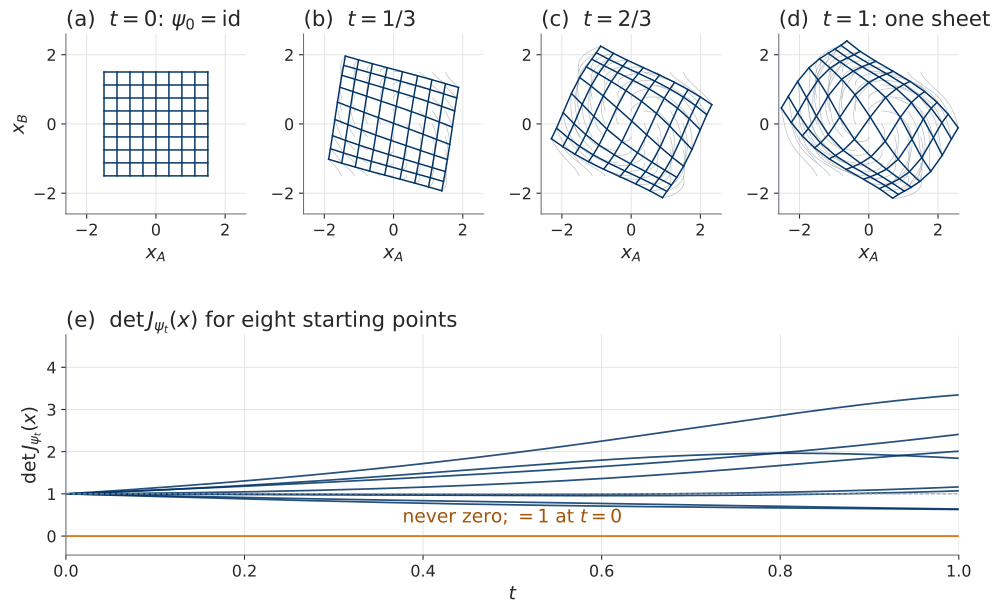
The flow map is not one map. It is a family \(\{\psi_t\}_{t \in [0, 1]}\) that starts at the identity and deforms continuously. Figure 1 shows the family for one field on the plane, and one number attached to it that §3 will use.
scripts/python/fig_u2_t1_flows.py.
Panel (e) is the picture behind the orientation statement of §3: the determinant of the flow map’s Jacobian is a continuous function of \(t\) that starts at \(1\) and never reaches zero. What it becomes as a function of the field is not computed here — that is the question on the board.
Why this matters later
U2.L1 profiles this model. U2.T2 puts a density on \(x_0\) and asks what \(\psi_t\) does to it, which is where the log-determinant returns. In U3 the same \(\psi_t\) is generated by a field chosen for a different reason, and the ODE limit of a residual stack returns once more, in the sampling discussion, as the identification of an Euler step with a residual step.
§3 — Well-posedness
Reference for this section: (Massaroli et al. 2020, sec. 2, “Well-posedness”) for the statement the source uses; the proof engine is U1.T2 §6 (PS1.5).
What could go wrong
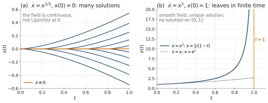
Equation 3 is an initial value problem, and the Definition of §2 assumed it has a unique solution on \([0, 1]\) for every \(x_0\). Two pictures show that the assumption is not free.
scripts/python/fig_u2_t1_wellposed.py.
Panel (a) is non-uniqueness: one initial condition, infinitely many solutions, so “the” flow map does not exist. Panel (b) is finite-time blow-up: the solution exists and is unique near \(t = 0\), but not on the whole interval, so \(\psi_1\) is not defined. The theorem below excludes exactly these two failures, with one hypothesis each.
Picard–Lindelöf, at the right strength
Let \(f \colon [0, 1] \times \mathbb{R}^{d} \to \mathbb{R}^{d}\) be continuous.
(Local.) If \(f\) is locally Lipschitz in \(x\), uniformly in \(t\) — for every bounded set \(B \subset \mathbb{R}^{d}\) there is \(L_B\) with \[ \lVert f(t, x) - f(t, y) \rVert \le L_B\, \lVert x - y \rVert \qquad \text{for all } t \in [0, 1],\; x, y \in B \] — then for every \(x_0\) there is a \(\delta > 0\) and a unique continuously differentiable solution of Equation 3 on \([0, \delta]\).
(Global, the course’s hypothesis.) If \(f\) is globally Lipschitz in \(x\), uniformly in \(t\) — one constant \(L\) serves all of \(\mathbb{R}^{d}\) — then for every \(x_0\) the solution exists, is unique, and is continuously differentiable on the whole of \([0, 1]\). The same conclusion holds under the weaker pair “locally Lipschitz + linear growth, \(\lVert f(t, x)\rVert \le a + b \lVert x \rVert\)”; global Lipschitz implies linear growth, and it is the hypothesis this course states.
The hypotheses name the two failures of Figure 2, one each. Panel (a)’s field is not Lipschitz at \(0\): the uniqueness hypothesis fails there, and in this example uniqueness does fail, as the drawn branches show. Panel (b)’s field is locally Lipschitz but not of linear growth (\(x^{2}\) grows faster than any line): the global hypothesis fails, and here the explicit solution shows that global existence fails too. Neither failure is forced by the missing hypothesis alone — the theorem is one-directional. \(\dot x = -x^{1/3}\) is not Lipschitz at \(0\) and has unique forward solutions; \(\dot x = -x^{3}\) grows faster than any line and exists on all of \([0, 1]\). A missing hypothesis removes the guarantee, not the conclusion.
The source states the global version in one line — a Lipschitz \(f_\theta\) gives, for each input, a unique solution defined on the whole interval (Massaroli et al. 2020, sec. 2) — and moves on. This page does the same in spirit, but the proof deserves a margin, because the students have already written it.
The proof engine, in the margin
U1.T2 §6 inverted a residual block \(f(x) = x + g(x)\) by turning \(f(x) = z\) into a fixed-point equation and applying the Banach fixed-point theorem on \(\mathbb{R}^{d}\). That is PS1.5. Picard–Lindelöf is the same argument on a different space.
Write the initial value problem as an integral equation: \[ x(t) = x_0 + \int_0^{t} f\big(\tau, x(\tau)\big)\,\mathrm{d}\tau, \qquad t \in [0, 1], \tag{5}\] which a continuous \(x\) satisfies if and only if it is a \(C^{1}\) solution of Equation 3 (differentiate one way, integrate the other). Call the right-hand side \((T x)(t)\). A solution is a fixed point of \(T\). Let \(L\) be the Lipschitz constant of \(f\) in \(x\). On \(C([0, 1]; \mathbb{R}^{d})\) use the weighted sup norm \(\lVert x \rVert_{w} = \sup_{t \in [0,1]} e^{-2Lt} \lVert x(t) \rVert\), which is equivalent to the plain sup norm (the weight lies between \(e^{-2L}\) and \(1\)), so the space is complete. The estimate that makes \(T\) a contraction is \[ \begin{aligned} \lVert (Tx - Ty)(t) \rVert &\le L \int_0^{t} \lVert x(\tau) - y(\tau) \rVert\,\mathrm{d}\tau \le L \int_0^{t} e^{2L\tau}\,\mathrm{d}\tau \cdot \lVert x - y \rVert_{w} \\ &\le \tfrac{1}{2}\, e^{2Lt}\, \lVert x - y \rVert_{w}, \qquad\text{so}\qquad \lVert Tx - Ty \rVert_{w} \le \tfrac{1}{2}\, \lVert x - y \rVert_{w} . \end{aligned} \tag{6}\]
| There — PS1.5 (U1.T2 §6) | Here — Picard–Lindelöf | |
|---|---|---|
| The space | \(\mathbb{R}^{d}\), Euclidean norm; complete | \(C([0, 1]; \mathbb{R}^{d})\), the norm \(\lVert \cdot \rVert_{w}\); complete |
| The map | \(T_z(x) = z - g(x)\) | \(T\) of Equation 5 |
| The contraction estimate | \(\operatorname{Lip}(T_z) = \operatorname{Lip}(g) < 1\) | \(\operatorname{Lip}(T) \le \tfrac{1}{2}\) in \(\lVert \cdot \rVert_{w}\) (Equation 6) |
| What buys the contraction | an architectural condition: the block’s Lipschitz constant must be below \(1\) | the weight \(e^{-2Lt}\): any finite \(L\) works, and nothing is asked of the size of \(L\) |
| The fixed point | \(x^{\ast}\) with \(x^{\ast} + g(x^{\ast}) = z\), i.e. \(f^{-1}(z)\) | \(x^{\ast}\) with \(x^{\ast} = T x^{\ast}\), i.e. the solution of Equation 3 on all of \([0, 1]\) |
| Uniqueness buys | \(f\) is a bijection of \(\mathbb{R}^{d}\) | two solutions through the same point at the same time coincide (used in §3, what a regular flow map cannot be) |
| The iteration | converges from any start (PS1.5(d), with a rate) | Picard iteration converges from any start; not used later in the course |
The local statement is the same argument on \(C([0, \delta]; \mathbb{R}^{d})\) with the plain sup norm and \(\delta L_B < 1\), after first checking that \(T\) maps a ball around the constant function \(x_0\) into itself for small \(\delta\). The linear-growth variant is the local statement plus an a-priori bound that keeps the solution inside a fixed ball on \([0, 1]\); it is not needed under the course’s hypothesis.
The one line to remember: the residual block needed \(L < 1\); the flow needs \(L < \infty\). That is the whole content of “continuous time relaxes the architectural constraint”, and it is exactly as strong as it sounds and no stronger — the field still needs a Lipschitz constant.
The standing regularity contract for U2
Two different things are asked of \(f_\theta\) in this unit, and they are easy to conflate.
Tier 1 — well-posedness. \(f_\theta\) is continuous in \((t, x)\) and globally Lipschitz in \(x\) uniformly in \(t\). This is what §3, Picard–Lindelöf needs, and it is all that existence, uniqueness and invertibility of \(\psi_t\) need.
Tier 2 — differential identities. For the adjoint method (§4) and for the divergence identities of U2.T2, \(f_\theta\) is in addition continuously differentiable in \(x\) and in \(\theta\), with \(\partial f_\theta / \partial x\) and \(\partial f_\theta / \partial \theta\) continuous. Under Tier 2 the flow map \(\psi_t\) is itself continuously differentiable in \(x_0\), with an invertible Jacobian, and \(t \mapsto J_{\psi_t}(x_0)\) is continuous (the standard theorem on differentiable dependence on initial conditions).
The course’s models use smooth activations (tanh, softplus) and satisfy both tiers. A ReLU network is Lipschitz and satisfies Tier 1; it is not \(C^{1}\), and an identity that needs Tier 2 does not hold for it as stated. The two roles are kept apart in every statement of this unit.
Invertibility by well-posedness, not for free
Under Tier 1, for \(t_0 < t_1\) in \([0, 1]\) the map \(\psi_{t_0 \to t_1}\) is a bijection of \(\mathbb{R}^{d}\) onto \(\mathbb{R}^{d}\), and its inverse is obtained by integrating the same equation \(\dot x = f_\theta(t, x)\) backward in time from \(t_1\) to \(t_0\). Both the map and its inverse are continuous (by Grönwall’s inequality, two solutions started \(\delta\) apart stay within \(\delta e^{L}\) of each other), so \(\psi_{t_0 \to t_1}\) is a homeomorphism. Under Tier 2 it is a diffeomorphism.
Proof. Injective: if \(\psi_{t_0 \to t_1}(x) = \psi_{t_0 \to t_1}(y)\), the two solutions pass through the same point at time \(t_1\); the initial value problem posed at time \(t_1\) (solved backward, which is the same theorem on the interval \([t_0, t_1]\) traversed in reverse) has a unique solution, so they coincide on \([t_0, t_1]\) and \(x = y\). Surjective: given \(y \in \mathbb{R}^{d}\), solve backward from \(y\) at time \(t_1\); the solution exists on \([t_0, t_1]\) by the global theorem, and its value at \(t_0\) is a preimage. The inverse is that backward solve. Continuity: if \(x, y\) solve the equation from \(x(t_0), y(t_0)\), then \(\lVert x(t) - y(t) \rVert \le \lVert x(t_0) - y(t_0) \rVert + L \int_{t_0}^{t} \lVert x - y \rVert\,\mathrm{d}\tau\), and Grönwall’s inequality gives \(\lVert x(t) - y(t) \rVert \le e^{L (t - t_0)} \lVert x(t_0) - y(t_0) \rVert\); the same bound holds for the backward solve. Under Tier 2 the Jacobians of \(\psi_{t_0 \to t_1}\) and of its inverse are inverse matrices, both continuous. \(\square\)
Two remarks, one about words and one about cost.
Words. “The inverse is the flow of \(-f\)” is a sentence one meets, and it is valid only after a time reversal. Set \(y(\tau) = x(t_1 - \tau)\) for \(\tau \in [0, t_1 - t_0]\). Then \(\dot y(\tau) = -\,f_\theta\big(t_1 - \tau, y(\tau)\big)\): a different non-autonomous field, read forward in the new clock \(\tau\). For an autonomous field the two sentences agree; for \(f_\theta(t, x)\) with genuine \(t\)-dependence, “run the same equation backward” is the correct one, and it is what a solver does when asked to integrate from \(t_1\) to \(t_0\).
Cost. Invertibility is now structurally automatic: no coupling pattern, no triangular Jacobian, no contraction condition on each block. It is not computationally free: the inverse is a numerical ODE solve, with its own step count. The unit of that cost is the one the course has carried since U0: the number of function evaluations, NFE, the number of times the solver asks \(f_\theta\) for its value. Both directions of the map — sampling and its inverse — pay in that currency.
What a regular flow map cannot be
U1.T2 §5 produced topology-obstruction-argument: a flow of that unit is a homeomorphism of \(\mathbb{R}^{d}\), so it preserves the topology of a support and cannot exactly reach a disconnected or lower-dimensional target. That statement stays true here, because \(\psi_1\) is a homeomorphism, and it keeps its U1 meaning and version. Today adds a different restriction, about which maps arise as flows at all, and records it separately so that U3 can cite the two without conflating them.
Let \(f\) satisfy Tier 1 and let \(\psi_t\) be its flow map.
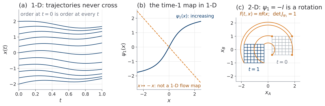
(i) One dimension: order is preserved. If \(d = 1\) and \(x_0 < y_0\), then \(\psi_t(x_0) < \psi_t(y_0)\) for every \(t \in [0, 1]\). Hence \(\psi_1\) is strictly increasing, and the reflection \(x \mapsto -x\) is not the time-1 map of any regular one-dimensional ODE.
(ii) Any dimension: orientation is preserved. Under Tier 2, \(\det J_{\psi_t}(x) > 0\) for every \(x\) and every \(t \in [0, 1]\). Hence a regular flow map is orientation-preserving; in particular \(x \mapsto -x\), whose Jacobian determinant is \((-1)^{d}\), is not a regular flow map in any odd dimension. In \(d = 2\) it is: \(-I\) is the rotation by \(\pi\), and it is \(\psi_1\) of the field \(f(t, x) = \pi R x\) with \(R\) the quarter-turn.
(iii) Scope. Orientation is a necessary condition, not a characterization. Which orientation-preserving diffeomorphisms are time-1 maps of a regular flow is a dimension-specific question, and no finer claim is made in this course.
Proof. (i) The functions \(t \mapsto \psi_t(x_0)\) and \(t \mapsto \psi_t(y_0)\) are continuous. If they took the same value at some \(t^{\ast}\), uniqueness for the initial value problem posed at time \(t^{\ast}\) (the same theorem, run backward to \(0\)) would force \(x_0 = y_0\). So their difference never vanishes on \([0, 1]\), and a continuous function that never vanishes keeps its sign: it is negative at \(t = 0\), so it is negative throughout. In words, two trajectories of a regular one-dimensional equation never cross, and their order at \(t = 0\) is their order at every \(t\). (ii) By the contract, \(t \mapsto \det J_{\psi_t}(x)\) is continuous on \([0, 1]\); it equals \(\det I = 1\) at \(t = 0\); and it never vanishes, because \(J_{\psi_t}(x)\) is invertible (§3, invertibility). A continuous function on an interval that never vanishes and is positive at one point is positive everywhere. The rotation claim is a computation: \(\dot x = \pi R x\) has solution \(x(t) = \exp(\pi t R) x_0\), and \(\exp(\pi R) = -I\). \(\square\)
scripts/python/fig_u2_t1_flows.py.
The one-dimensional example is the “crossing trajectories” problem of (Massaroli et al. 2020, sec. 5), read in exactly the order-preservation sense of (i); the source uses it to motivate conditioning the field on the input, which is literature texture and not course content. The picture to keep is Figure 3(c): what is impossible on the line is a rotation on the plane.
The two costs, version 2, annotated
The left board gets one new row today. It is not version 3 — that is U2.T2’s, when the cells change — but the row that records what this session has resolved and what it has not.
| Family | Density | Sampling | Trick, and its price |
|---|---|---|---|
| NICE / RealNVP | exact, triangular | direct | coupling; depth |
| Glow | exact | direct | mixing, multi-scale |
| MAF | parallel | sequential | AR, data side |
| IAF | sequential | parallel | AR, source side |
| Residual flow | direct; series log-det | iterative | contraction, traces |
| Neural ODE | inverse: ODE solve / NFE; \(\log\lvert\det J\rvert\): ??? | ODE solve / NFE | no inverse layer to design; Lipschitz field |
Read the new row against the others. The architectural inverse constraint is resolved: nothing about the layer has to be designed for invertibility, only the field’s regularity. The runtime is an ODE solve in both directions, priced in NFE. And the log-determinant cell is open; it is the question on the board, and it is circled at the close.
Why this matters later
U2.T2 opens on the open cell. The two-tier contract is what lets it state the divergence identities without re-deriving regularity. The continuous-flow-map restriction is cited by U3.T1 beside, not inside, U1’s support result, and returns in the U7 synthesis.
§4 — The adjoint method
References for this section: (Massaroli et al. 2020, App. A.1) (the Lagrangian derivation, which this section follows after translation); (Chen et al. 2018, sec. 2 and App. B) (the historical statement, the augmented-state algorithm, and a proof by a limit argument).
The setup, and one letter
Fix \(x_0\), let \(x\) solve Equation 3 under Tier 2, and let a loss depend on the endpoint: \[ \ell(\theta) = L\big(x(1)\big), \qquad L \in C^{1}(\mathbb{R}^{d}; \mathbb{R}). \tag{7}\] Training needs \(\mathrm{d}\ell / \mathrm{d}\theta \in \mathbb{R}^{1 \times p}\). The obvious route is to unroll the solver’s arithmetic and backpropagate through every step, storing every intermediate state; §5 prices it. The adjoint method computes the same object without storing what the solver did. Throughout, cotangents are row vectors, the convention of the bootcamp’s VJP: the adjoint state is written \(a^{\top}(t) \in \mathbb{R}^{1 \times d}\).
One letter, before the derivation. In this course \(\mathcal{L}\) is the letter of a training loss (\(\mathcal{L}_{\mathrm{FM}}\) later). Today \(\mathcal{L}\) is not a loss. It is the perturbed functional, the Lagrangian of the derivation below, and the loss is \(\ell\). The two coincide in value along trajectories — that is the whole trick — but they are different functions of their arguments, and the notation keeps them apart. The pinned problem set uses the same two letters. And the roman \(L\) of this section is the terminal loss function, not the Lipschitz constant of §3.
Step 0 — the discrete ancestor
Backpropagation pushes a cotangent backward through a composition of maps. The rule is two lines, and it is the only bootcamp result this page uses (proved in the bootcamp, U0.T1, as the artifact vjp-composition-proof; here it is restated in full).
For a composition \(F = f_K \circ \cdots \circ f_1\) of \(K\) maps, with intermediates \(x^{k} = f_k(x^{k-1})\), \(x^{0} = x\), and a cotangent \(v^{\top}\) on the output, \[ \begin{aligned} v_K^{\top} &= v^{\top}, \qquad v_{k-1}^{\top} = v_k^{\top}\, J_{f_k}\big(x^{k-1}\big) \quad (k = K, \dots, 1), \\ &\text{gives}\qquad v_0^{\top} = v^{\top} J_F(x). \end{aligned} \] (The bootcamp writes the composed map as \(h\) and the depth as \(L\); here \(h\) is the Euler step and \(L\) the loss, so the letters are \(F\) and \(K\).) Each step is a vector–Jacobian product, computable at about the cost of one evaluation of \(f_k\) without forming \(J_{f_k}\).
Read the recursion as a discrete-time equation for a row vector: at each layer the cotangent is multiplied on the right by the layer’s Jacobian. Now let the layers be the Euler steps of Equation 1: the \(k\)-th layer maps \(x_{k-1}\) to \(x_k\), so \(f_k(x) = x + h f(t_{k-1}, x)\) and \(J_{f_k}(x_{k-1}) = I + h\, \partial f / \partial x(t_{k-1}, x_{k-1})\) (the \(x^{k}\) of the box are the \(x_k\) of the stack), and the recursion reads \[ v_{k-1}^{\top} = v_k^{\top} + h\, v_k^{\top}\, \frac{\partial f}{\partial x}(t_{k-1}, x_{k-1}), \] an explicit Euler step of an equation for the row vector, taken backward in time. As \(h \to 0\) it wants to become \(\dot a^{\top} = -\,a^{\top}\, \partial f / \partial x\). That is the adjoint equation, and the derivation below reaches it by a different road, one that makes no limit argument. The adjoint state is the running VJP. Whether the discrete recursion is exactly the adjoint of the discrete map is PS2.1(g); it is, and the sentence you will write there is this session’s thesis.
The derivation, in full
The live session performs this derivation on the board with three gaps, labelled G1–G3, drawn as empty boxes and assigned as PS2.1. These notes fill the boxes, because this box is the citable object of the unit.
Setting. \(f_\theta\) satisfies Tier 2 of §3, the standing contract, \(x_0\) does not depend on \(\theta\), \(x\) solves Equation 3, and \(\ell(\theta) = L(x(1))\) with \(L \in C^{1}\). Write \(A(t) = \partial f_\theta / \partial x\,(t, x(t)) \in \mathbb{R}^{d \times d}\) and \(B(t) = \partial f_\theta / \partial \theta\,(t, x(t)) \in \mathbb{R}^{d \times p}\); both are continuous in \(t\).
Step 1 — the perturbed functional. Fix \(\theta_0\). For any continuously differentiable \(a \colon [0, 1] \to \mathbb{R}^{d}\), chosen once and held fixed as a function of \(t\) alone, define \[ \mathcal{L}(\theta) = \ell(\theta) - \int_0^{1} a^{\top}(t)\,\big[\dot x(t) - f_\theta\big(t, x(t)\big)\big]\,\mathrm{d}t . \tag{8}\] The bracket is identically zero because \(x\) solves the equation, for every \(\theta\). So \(\mathcal{L}(\theta) = \ell(\theta)\) for all \(\theta\), and in particular \(\mathrm{d}\mathcal{L}/\mathrm{d}\theta = \mathrm{d}\ell/\mathrm{d}\theta\) at \(\theta_0\), whatever \(a\) is. [This is G2, first half.]
Step 2 — integration by parts. [G1.] Since \(a\) and \(x\) are \(C^{1}\), \[ \int_0^{1} a^{\top}\dot x\,\mathrm{d}t = a^{\top}(1)\,x(1) - a^{\top}(0)\,x(0) - \int_0^{1} \dot a^{\top} x\,\mathrm{d}t, \] hence \[ \begin{aligned} \mathcal{L}(\theta) = L\big(x(1)\big) &- a^{\top}(1)\,x(1) + a^{\top}(0)\,x_0 \\ &+ \int_0^{1} \Big[\dot a^{\top}(t)\,x(t) + a^{\top}(t)\,f_\theta\big(t, x(t)\big)\Big]\mathrm{d}t . \end{aligned} \tag{9}\]
Step 3 — differentiate, and collect the sensitivity. Under Tier 2 the solution depends continuously differentiably on \(\theta\) (differentiable dependence on parameters), so \(S(t) = \mathrm{d}x(t)/\mathrm{d}\theta \in \mathbb{R}^{d \times p}\) exists and is continuous in \(t\), and \(S(0) = 0\) because \(x_0\) does not depend on \(\theta\). Differentiating Equation 9 term by term (the \(\theta\)-derivative of the integrand is jointly continuous in \((t, \theta)\) — which is what differentiable dependence on parameters provides — so differentiation passes under the integral): \[ \begin{aligned} \frac{\mathrm{d}\mathcal{L}}{\mathrm{d}\theta} &= \Big[\frac{\partial L}{\partial x}\big(x(1)\big) - a^{\top}(1)\Big]\, S(1) \\ &\quad + \int_0^{1} \Big[\dot a^{\top}(t) + a^{\top}(t)\,A(t)\Big]\, S(t)\,\mathrm{d}t + \int_0^{1} a^{\top}(t)\, B(t)\,\mathrm{d}t . \end{aligned} \tag{10}\] The three groups are: what multiplies the unknown \(S(1)\); what multiplies the unknown \(S(t)\) under the integral; and what involves no sensitivity at all. The term \(a^{\top}(0) S(0)\) vanished.
Step 4 — spend the free choice. [G2, second half.] Choose \(a\) to be the solution of the linear final-value problem \[ \dot a^{\top}(t) = -\,a^{\top}(t)\, A(t), \qquad a^{\top}(1) = \frac{\partial L}{\partial x}\big(x(1)\big), \tag{11}\] which exists, is unique and is \(C^{1}\) on \([0, 1]\) by §3, Picard–Lindelöf (a linear equation with a continuous coefficient matrix is globally Lipschitz with constant \(\Lambda = \sup_t \lVert A(t) \rVert\); the letter \(L\) is the loss here). Evaluate Equation 10 at \(\theta = \theta_0\): with this \(a\) both sensitivity groups vanish for every \(t\), whatever \(S(t)\) is. The choice is legitimate because Step 1 holds for every fixed \(a\), and this \(a\) — built from the trajectory at \(\theta_0\) — is one such. A free choice, spent wisely: the same proof taste as the projection Lemma (UP.T1), and no formal connection claimed.
Step 5 — what survives. \[ \boxed{\; \begin{aligned} \frac{\mathrm{d}\ell}{\mathrm{d}\theta} &= \int_0^{1} a^{\top}(t)\, \frac{\partial f_\theta}{\partial \theta}\big(t, x(t)\big)\,\mathrm{d}t, \\ \dot a^{\top} &= -\,a^{\top}\,\frac{\partial f_\theta}{\partial x}(t, x), \qquad a^{\top}(1) = \frac{\partial L}{\partial x}\big(x(1)\big). \end{aligned} \;} \tag{12}\] This is the theorem, and the derivation is complete. \(\square\)
Under the setting of Box U2.T1-3, the gradient of \(\ell(\theta) = L(x(1))\) is given by Equation 12: \(a^{\top}\) solves the adjoint equation backward from its terminal value, and the gradient is the time integral of \(a^{\top}\) against \(\partial f_\theta / \partial \theta\) along the trajectory. Moreover \(a^{\top}(t) = \mathrm{d}\ell / \mathrm{d}x(t)\), the sensitivity of the loss to the state at time \(t\) — the running VJP.
The last sentence is not proved by the Lagrangian route as written; it is what (Chen et al. 2018, App. B) proves first, by writing the chain rule for an \(\varepsilon\)-step of the flow and letting \(\varepsilon \to 0\), and it is checked on the worked example below. Both readings are true; the Lagrangian gives the gradient formula without a limit, the limit argument gives the interpretation.
Implementation — the augmented backward solve
[G3.] The theorem asks for an integral along the trajectory, evaluated backward in time. Implement it as one more state: the parameter adjoint \(a_\theta(t) \in \mathbb{R}^{p}\) with \[ \dot a_\theta^{\top}(t) = -\,a^{\top}(t)\, \frac{\partial f_\theta}{\partial \theta}\big(t, x(t)\big), \qquad a_\theta(1) = 0 . \tag{13}\] Then solve the augmented system in \((x, a, a_\theta)\), of dimension \(2d + p\), backward from \(t = 1\) to \(t = 0\), starting from \(\big(x(1),\; \partial L/\partial x(x(1))^{\top},\; 0\big)\) with dynamics \(\big(f_\theta,\; -A^{\top} a,\; -B^{\top} a\big)\), and read \[ \frac{\mathrm{d}\ell}{\mathrm{d}\theta} = a_\theta(0)^{\top}. \tag{14}\] This is (Chen et al. 2018, Algorithm 1), in course notation. The state \(x(t)\) is reconstructed by integrating its own equation backward beside \(a\); it is not stored. Verifying that \(a_\theta(0)\) equals the boxed integral is PS2.1(e) — one line, once you see which direction the integral runs.
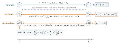
Two facts about the right-hand side of the backward solve. Each of \(a^{\top} \partial f / \partial x\) and \(a^{\top} \partial f / \partial \theta\) is a vector–Jacobian product, the primitive of Step 0: reverse-mode autodiff computes each at about the cost of one evaluation of \(f_\theta\) and never forms a Jacobian. So every RHS evaluation of the backward solve costs a small constant multiple of a forward one — and the NFE of the backward pass is a second bill, on top of the forward one.
Return to \(f_\theta(t, x) = -\theta x\) on \(\mathbb{R}\), \(x(0) = x_0\), with \(L(x) = \tfrac{1}{2} x^{2}.\)
Directly. \(x(1) = x_0 e^{-\theta}\), so \(\ell(\theta) = \tfrac{1}{2} x_0^{2} e^{-2\theta}\) and \(\mathrm{d}\ell/\mathrm{d}\theta = -x_0^{2} e^{-2\theta}\).
By the adjoint. \(\partial f/\partial x = -\theta\), so Equation 11 reads \(\dot a = \theta a\) with \(a(1) = L'(x(1)) = x_0 e^{-\theta}\), whence \(a(t) = x_0 e^{-\theta} e^{\theta (t - 1)} = x_0 e^{\theta(t - 2)}\). And \(\partial f/\partial \theta = -x(t) = -x_0 e^{-\theta t}\). So \[ \begin{aligned} \int_0^{1} a(t)\, \frac{\partial f}{\partial\theta}\,\mathrm{d}t &= -x_0^{2} \int_0^{1} e^{\theta(t - 2)} e^{-\theta t}\,\mathrm{d}t \\ &= -x_0^{2} e^{-2\theta} \int_0^{1} \mathrm{d}t = -x_0^{2} e^{-2\theta} . \end{aligned} \] The two agree. The interpretation, checked: the loss as a function of the state at time \(t\) is \(\ell = \tfrac{1}{2}\, x(t)^{2} e^{-2\theta(1 - t)},\) whose derivative in \(x(t)\) is \(x(t) e^{-2\theta(1 - t)} = x_0 e^{-\theta t} e^{-2\theta + 2\theta t} = x_0 e^{\theta(t - 2)} = a(t)\). The adjoint is the running sensitivity.
The punchline, said plainly
For a fixed number of requested output times (here one, \(t = 1\)), the continuous-adjoint implementation stores a constant amount of state with respect to the number of solver steps: \(x(1)\), \(a\), \(a_\theta\), and whatever the solver needs for its current step. Direct backpropagation stores every intermediate state the solver produced. That is the memory technology, and it is what U2.L1 measures.
The price is two things. Another numerical solve, of a system of dimension \(2d + p\), with its own NFE. And a gradient that is an approximation of the exact-solution gradient, obtained by discretizing the adjoint equation, rather than the exact gradient of the discretized forward map — optimize-then-discretize. §5 reads that distinction slowly.
Bonus statement — the generalized adjoint
Let the loss also charge the trajectory: \[ \ell(\theta) = L\big(x(1)\big) + \int_0^{1} l\big(t, x(t), \theta\big)\,\mathrm{d}t, \qquad l \in C^{1} . \] Then the adjoint equation gains a source term and the gradient gains a direct term: \[ \begin{aligned} \dot a^{\top} &= -\,a^{\top}\,\frac{\partial f_\theta}{\partial x} - \frac{\partial l}{\partial x}, \qquad a^{\top}(1) = \frac{\partial L}{\partial x}\big(x(1)\big), \\ \frac{\mathrm{d}\ell}{\mathrm{d}\theta} &= \int_0^{1} \Big[a^{\top}\,\frac{\partial f_\theta}{\partial \theta} + \frac{\partial l}{\partial \theta}\Big]\mathrm{d}t . \end{aligned} \] Proposition 1 of Massaroli et al. (2020) states and proves the case \(l = l(t, x)\) with no explicit dependence on \(\theta\), where the second term is absent; the \(\partial l / \partial \theta\) term is the direct contribution when the integrand depends on the parameters. That case is not academic: a regularizer that penalizes the learned field itself along the trajectory (U2.T2 meets one) depends on \(\theta\) explicitly, and “integral loss” is then not merely an extra state derivative.
Why this matters later
The adjoint is (i) the memory technology that makes U2.L1’s profiling experiment meaningful, (ii) the cost centre whose NFE bill U2.L2 measures — the pain U3 exists to remove — and (iii) the completion of the bootcamp’s foreshadow, “backprop is the discrete ancestor of the adjoint”. The generalized statement pays off in U2.T2 (regularization) and, quietly, in the U6 reading track on integral losses.
§5 — Backprop through the solver, or the adjoint
Reference for this section: (Kidger 2022, sec. 5.1) (“Backpropagation through ODEs”: discretise-then-optimise, optimise-then-discretise, reversible solvers), which treats everything here at greater depth.
The two strategies, in one table
| Memory | Compute | Correctness | |
|---|---|---|---|
| Direct backprop through the solver (discretize → optimize) | every stored solver state: grows with the number of steps | one forward solve, then one reverse sweep of VJPs over the recorded operations, about the cost of the forward solve | for a fixed-step solver, the exact gradient of the executed discrete map, up to round-off |
| Continuous adjoint (optimize → discretize) | \(O(1)\) in the number of solver steps, at a fixed number of requested output times | a second solve, of the augmented system of dimension \(2d + p\), each RHS call paying one \(f_\theta\) evaluation plus VJPs — a second NFE bill | an approximation of the exact-solution gradient: two discretizations (forward, backward), and the backward reconstruction can drift |
Correctness, read slowly
The correctness column is where the two strategies differ in kind, not in degree, and the distinction has a name on each side.
Discretize, then optimize. A fixed-step solver computes a specific composition of arithmetic operations — \(K\) Euler steps, or \(K\) Runge–Kutta stages — and direct autodiff differentiates that composition. The result is the exact gradient of the function the computer actually evaluated. It is not the gradient of the exact solution’s loss; it is the gradient of the discretized solution’s loss, and the two differ by the discretization error’s own derivative. For an adaptive solver the statement weakens: the step controller makes decisions (accept, reject, halve, double) that depend on the state, autodiff treats those decisions as constants, and the “exact gradient of the discretization” becomes a statement about the executed trace — locally valid, not globally smooth.
Optimize, then discretize. The continuous adjoint first derives the gradient of the exact solution’s loss (that is Equation 12) and then discretizes the adjoint equation with a solver. The gradient it returns is close to the true gradient when both solves are accurate, and it is not the gradient of anything the forward solver computed. Two discretization errors enter, and in addition the backward pass reconstructs \(x(t)\) by integrating the forward equation backward, which is stable only when the reversed dynamics are.
Neither strategy is “the correct one”. A gradient that is exact for the wrong function and a gradient that is approximate for the right function are both approximations of what one wants, and which is better is an empirical question about a given problem, solver and tolerance. U2.L1 asks it with a table.
The asterisk under invertibility
§3, invertibility proved that a regular flow is invertible by running the equation backward. Nothing in that proof says the backward solve is numerically well behaved, and often it is not: when the forward flow contracts, the backward flow expands, and any error at \(t = 1\) is amplified on the way to \(t = 0\).
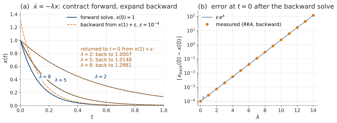
scripts/python/fig_u2_t1_adjoint.py.
The figure shows one mechanism on one linear field. It does not say that every adjoint solve drifts, and it measures no gradient; gradient fidelity on a trained model is U2.L1’s measurement. What it says is why that measurement has to exist: the direction of the solve decides whether errors shrink or grow, and the adjoint always solves in the direction the forward pass did not.
Mitigations, named and not oversold. Tighter tolerances on the backward solve, which cost NFE. Direct backpropagation, when the problem is small enough to store. Checkpointing and hybrid schemes, which store a few states along the forward trajectory and reconstruct only between them, trading memory for a bounded reconstruction length — in systems that support them. torchdiffeq (Chen 2018) offers the continuous adjoint as odeint_adjoint; Diffrax (Kidger 2021) makes recursive checkpointing its default route and offers the continuous adjoint as a contrast, and U2.L1 uses exactly that contrast. None of these is a theorem; each is an engineering choice with a bill.
The plot you will make
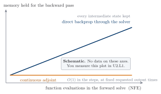
In U2.L1 you will produce this plot yourselves, on a small classifier where nothing hurts yet, and compare it against this schematic. The plot stays session-local to U2.L1 by decision; the instrument that makes it — an NFE counter, a memory probe, a gradient-fidelity check — is what the lab installs, so that U2.L2 can point it at a generative model.
Why this matters later
The exact-gradient-of-the-discretization distinction returns when U3 discusses solver error in sampling: there it is error in samples, here in gradients, the same taxonomy. The drift remark is the honest numerical asterisk under the structurally automatic invertibility of §3.
§6 — Close: PS2.1 assigned, the question that stays open
PS2.1, assigned at the board
PS2.1 is assigned the moment the boxed theorem and the three gap boxes are both visible. The gaps are the assignment.
Setting: \(\dot x = f_\theta(t, x)\), \(x(0) = x_0\), \(\ell = L(x(1))\), \(f_\theta\) continuously differentiable, Lipschitz in \(x\).
- (a) Define the perturbed functional \(\mathcal{L}\) with multiplier \(a(t)\) and justify \(\mathrm{d}\ell/\mathrm{d}\theta = \mathrm{d}\mathcal{L}/\mathrm{d}\theta\) for every choice of \(a\). [= G2, part 1]
- (b) Carry out the integration by parts, tracking boundary terms at \(t = 0\) and \(t = 1\) explicitly. [= G1]
- (c) Differentiate \(\mathcal{L}\) w.r.t. \(\theta\) and collect all terms containing \(\mathrm{d}x/\mathrm{d}\theta\). Explain why \(\mathrm{d}x(0)/\mathrm{d}\theta = 0\).
- (d) Exhibit the choice of final-value problem for \(a(t)\) that annihilates every \(\mathrm{d}x/\mathrm{d}\theta\) term; conclude the adjoint sensitivity theorem. [= G2, part 2]
- (e) Derive the augmented-state implementation: show that \(a_\theta(0)\) as defined in lecture equals the boxed integral. [= G3]
- (f) Bonus. Extend (a)–(d) to \(\ell = L(x(1)) + \int_0^{1} l(t, x(t), \theta)\,\mathrm{d}t\). Recover both the \(-\partial l/\partial x\) term in the adjoint ODE and the direct \(\partial l/\partial\theta\) contribution to \(\mathrm{d}\ell/\mathrm{d}\theta\) (Massaroli et al. 2020, Prop. 1); attached PDF only after attempting.
- (g) Bonus. Euler-discretize the forward ODE with step \(h\) and show the adjoint recursion at the discrete points is exactly reverse-mode autodiff through the unrolled steps (the VJP identity from lecture). Conclude in one sentence in what precise sense “the adjoint is backprop’s continuum limit.”
Assigned today; released with PS2. Part (g)’s concluding sentence is the session’s thesis, and it is yours to write — it is not in these notes.
The board at the close
The left board is Table 2 with the log-determinant cell circled. The right board is Equation 12 beside PS2.1 (a)–(g), each part annotated with its G-number. Top right, not erased: what does \(\log\lvert\det J\rvert\) become in continuous time?
The last sentence of the session, verbatim:
We can now build continuous-depth invertible maps and differentiate them without storing every solver step. What we cannot yet do is account for their density change cheaply. The lab measures the numerical bill; U2.T2 finds out what \(\log\lvert\det J\rvert\) became.
§7 — Exercises, with answers
These are short, and none of them is part of PS2.1.
- A linear flow. Let \(f(t, x) = M x\) on \(\mathbb{R}^{2}\) with a constant matrix \(M\). Write \(\psi_t\) in closed form and its Jacobian. Check, without any formula for the determinant, the three facts the orientation statement of §3, what a regular flow map cannot be uses — continuity in \(t\), value \(1\) at \(t = 0\), never zero — and find an \(M\) that gives \(\psi_1 = -I\), with \(\det J_{\psi_1}\) computed directly.
- Time reversal. Let \(x\) solve \(\dot x = f(t, x)\) on \([t_0, t_1]\) and set \(y(\tau) = x(t_1 - \tau)\). Show that \(y\) solves \(\dot y(\tau) = -f(t_1 - \tau, y(\tau))\) on \([0, t_1 - t_0]\), and explain in one sentence why “the flow of \(-f\)” is the wrong phrase for a field with genuine \(t\)-dependence.
- The scalar adjoint with another loss. Repeat the worked example of §4, the augmented backward solve with \(L(x) = x\) (so \(\ell(\theta) = x(1)\)). Compute \(\mathrm{d}\ell/\mathrm{d}\theta\) directly and by the adjoint, and verify \(a(t) = \mathrm{d}\ell/\mathrm{d}x(t)\).
Answer to Exercise 1
\(\psi_t(x_0) = \exp(tM)\, x_0\) (the unique solution of \(\dot x = Mx\), \(x(0) = x_0\)), so \(J_{\psi_t} = \exp(tM)\) for every \(x_0\). The three facts: \(t \mapsto \exp(tM)\) is continuous (a power series in \(t\)); \(\exp(0) = I\) has determinant \(1\); and \(\exp(tM)\) is invertible for every \(t\), with inverse \(\exp(-tM)\), so its determinant is never zero. A continuous, never-zero function equal to \(1\) at \(0\) is positive: the orientation statement, checked on this family. For \(\psi_1 = -I\) one needs \(\exp(M) = -I\); \(M = \pi R\) with \(R = \bigl(\begin{smallmatrix} 0 & -1 \\ 1 & 0 \end{smallmatrix}\bigr)\) works, because \(\exp(t \pi R)\) is the rotation by the angle \(\pi t\), and the rotation by \(\pi\) is \(-I\). Directly, \(\det J_{\psi_1} = \det(-I) = (-1)^{2} = 1\), and at every \(t\) the rotation matrix has determinant \(\cos^{2}(\pi t) + \sin^{2}(\pi t) = 1\), as Figure 3(c) measured. (Nothing here says what \(\det J_{\psi_t}\) is as a function of a general field — that is the open question, and it stays open.)
Answer to Exercise 2
By the chain rule, \(\dot y(\tau) = -\dot x(t_1 - \tau) = -f\big(t_1 - \tau, x(t_1 - \tau)\big) = -f\big(t_1 - \tau, y(\tau)\big)\), and \(y(0) = x(t_1)\), \(y(t_1 - t_0) = x(t_0)\). The field on the right is \(-f\) evaluated at the reversed time \(t_1 - \tau\), not at \(\tau\); for an autonomous \(f\) the two agree, and for a field with genuine \(t\)-dependence “the flow of \(-f\)” names a different equation. “Integrate the same equation backward” is the phrase that is always right.
Answer to Exercise 3
Directly: \(\ell(\theta) = x_0 e^{-\theta}\), so \(\mathrm{d}\ell/\mathrm{d}\theta = -x_0 e^{-\theta}\). By the adjoint: \(a(1) = L'(x(1)) = 1\), \(\dot a = \theta a\), so \(a(t) = e^{\theta(t - 1)}\); and \(\partial f/\partial\theta = -x_0 e^{-\theta t}\), so \(\int_0^{1} a\,\partial f/\partial\theta\,\mathrm{d}t = -x_0 e^{-\theta}\int_0^{1} \mathrm{d}t = -x_0 e^{-\theta}\). Interpretation: \(\ell\) as a function of \(x(t)\) is \(x(t) e^{-\theta(1 - t)}\), whose derivative in \(x(t)\) is \(e^{-\theta(1 - t)} = e^{\theta(t - 1)} = a(t)\).
Reading the board
| On the board | Status |
|---|---|
| Residual steps \(\to\) an ODE | Made precise (§2), with the honest caveat: the limit of this stack, with a shared \(\theta\); a generic ResNet’s limit is a parameter path \(\theta(t)\). |
| Does the solution exist, and is it unique? | Yes, under a Lipschitz field (§3, Picard–Lindelöf; proof engine = PS1.5’s Banach argument). Two tiers of regularity recorded for the unit. |
| Is the map invertible? | Structurally yes, computationally an ODE solve (§3). A regular flow map is orientation-preserving and, in 1-D, order-preserving (continuous-flow-map-restriction). |
| How do we differentiate through a solver? | The adjoint sensitivity theorem (§4, adjoint-derivation): \(O(1)\) memory in solver steps, at the price of a second solve and an optimize-then-discretize gradient. Gaps G1–G3 = PS2.1. |
| The two costs | Version 2, annotated (Table 2): the Neural ODE row, with its inverse resolved and its log-determinant open. |
| What does \(\log\lvert\det J\rvert\) become in continuous time? | Open. U2.T2. |
Where this page reappears
| From this page | Reappears in |
|---|---|
| The Neural ODE and its flow map, §2 | U2.L1 (the object profiled); U2.T2 (the object whose density is tracked); U3.T1 (\(\psi_t\) generated by a different field) |
| The honest caveat, §2 | nowhere else — it is here so that no later session overclaims |
| Picard–Lindelöf and the two-tier contract, §3 | U2.T2 (the divergence identities assume Tier 2 without re-deriving it); every later use of “regular field” |
| Invertibility by backward solve, §3 | U2.T2 (data \(\to\) base solves); U3.T3 (samplers as backward and forward solves) |
continuous-flow-map-restriction, §3 |
U3.T1 (cited beside, not inside, topology-obstruction-argument); U7.W2 |
two-costs-table v2 annotated, Table 2 |
U2.T2 (v3, where the cells change); U3.L1 |
adjoint-derivation, Box U2.T1-3 |
PS2.1; U2.L1 (“the method you are profiling is Box U2.T1-3”); U2.T2 and U2.L2 (cited, not re-derived); U3.T3 (one citation, in the solver-error discussion) |
| The generalized adjoint, §4 | U2.T2 (regularization); U6 Track A reading |
| The 2×3 table, Table 3 | U2.L1 (the gradient-fidelity table); U3.T3 (the same taxonomy for samples) |
| The drift picture, Figure 5 | U2.L1 (the adjoint-vs-checkpointing contrast in Diffrax) |
Next session
The next session is the lab (U2.L1): solvers and adjoints in practice — NFE, wall-clock, memory and gradient fidelity measured on a small Neural ODE classifier, with the memory plot of Figure 6 made with real numbers. The theory session after it (U2.T2) opens on the circled cell.
Before then: PS2.1 (§6) is assigned today. For the numerics of adjoints beyond this course — reversible solvers, the structure of adaptive step controllers, and what to do when the backward solve drifts — (Kidger 2022, ch. 5) is the reference, and it is optional.
References
Footnotes
Both papers write the integration variable of a Neural ODE as “depth”. (Massaroli et al. 2020) calls it \(s \in S\) and the state \(z(s)\); (Chen et al. 2018) calls it \(t \in [t_0, t_1]\) and the state \(z(t)\). In this course the variable is \(t \in [0, 1]\) and the state is \(x(t)\), always. The letter \(s\) is reserved by L1 §4 for a second clock that a later unit introduces, and never appears as a depth variable in course materials; the letter \(z\) is reserved for VAE latents. The literature uses \(s\) and \(t\) for depth interchangeably; we fix \(t\) and reserve \(s\). The dummy variable of an integral over time is \(\tau\).↩︎
U1.T2, §7, the figure “the stack converges as \(h \to 0\)”: endpoint error \(0.60\) at \(K = 2\) down to \(0.0012\) at \(K = 1024\), every halving ratio between \(1.91\) and \(2.03\).↩︎