U2.T1 — Neural ODEs and the Adjoint Method

Flow-Based Generative Models · UFRJ · 2026.2

01From residual steps to a flow

The question on the board

U1.T2 ended on a residual stack with a step size, and on one question:

What does \(\log\lvert\det J\rvert\) become in continuous time?

Today pays the first half of that debt, and leaves the question where it is:

Today	Not today
residual steps \(\to\) an ODE, honestly	the log-determinant
the flow exists, is unique, is invertible	any density
how to differentiate through a solver	any divergence

Zero to two minutes. BOARD 1 (left, persistent): U1.T2’s two-costs table v2, redrawn. BOARD 3 (right, top): the log-det question, rewritten now, and not erased at the close. Say the joint-audience sentence once: this session depends on U1.T2 and UP.T1, and on nothing from the bootcamp; the one bootcamp callback, the VJP composition rule, is on the slide in full when it comes.

The two costs, version 2

Family	Density	Sampling	Trick, and its price
NICE / RealNVP	exact, triangular	direct	coupling; depth
Glow	exact	direct	mixing, multi-scale
MAF	parallel	sequential	AR, data side
IAF	sequential	parallel	AR, source side
Residual flow	direct; series log-det	iterative	contraction, traces

Every row pays with an architectural constraint: a coupling, a mixing layer, an autoregressive (AR) ordering, a contraction. What if depth \(\to \infty\)?

Two to four minutes. Point at the empty space under the last row: one row is added today, at the end of the well-posedness block, and it will have a question mark in it.

A residual stack with a step size

Put \(h = 1/K\) in front of each residual branch, and let the branch depend on \(t_k = k h\):

\[ x_{k+1} = x_k + h\, f(t_k, x_k), \qquad k = 0, \dots, K-1 . \]

This is forward Euler for \(\dot x = f(t, x)\), \(x(0) = x_0\), \(t \in [0, 1]\) — the course’s f(t, x), time first. U1.T2 measured that the stack’s output converges as \(h \to 0\) (error halves when \(h\) halves).

What U1.T2 did not say: what the limit is; when it exists; whether it is unique; whether \(x_0 \mapsto x(1)\) is invertible; how to differentiate through it. That is today.

Four to seven minutes. BOARD 2 (centre, rolling): the Euler step and the ODE under it. Standalone phrasing: nobody needs to have seen U1.T2’s figure to follow. Say “time first” out loud once.

The model

Let \(f_\theta \colon [0,1] \times \mathbb{R}^{d} \to \mathbb{R}^{d}\) be a network with parameters \(\theta \in \mathbb{R}^{p}\), and suppose \[ \dot x(t) = f_\theta\big(t, x(t)\big), \qquad x(0) = x_0 \] has a unique solution on \([0, 1]\), and so does the same equation started from any \(x(t_0) = x\) with \(t_0 \in [0, 1]\) (the well-posedness block says when). The flow map is \(\psi_t(x_0) = x(t)\), with \(\psi_0 = \mathrm{id}\); the Neural ODE is \(x_0 \mapsto \psi_1(x_0)\). For \(t_0 < t_1\), \(\psi_{t_0 \to t_1}\) carries the state at \(t_0\) to the state at \(t_1\).

Seven to eight minutes. Read the definition once, slowly; the three things to notice are the next slide.

The model, read three ways

• Depth became the integration variable: no layer \(k\), only a time \(t\).
• One \(\theta\) serves the whole interval.
• \(\psi_t\) is the course symbol table’s symbol (L1 §4). Chosen with the future in mind: in U3 it is generated by a different kind of field. Today it is only the solution map.

Eight to ten minutes. The three bullets in that order. The gray sentence is the only gesture toward U3; nothing more is said about it today.

Worked example: a flow map in closed form

\(d = 1\), \(f_\theta(t, x) = -\theta x\), \(\theta > 0\). Then \(\dot x = -\theta x\), \(x(0) = x_0\) gives \(x(t) = x_0 e^{-\theta t}\): \[ \psi_t(x_0) = e^{-\theta t} x_0, \qquad \psi_0 = \mathrm{id}, \qquad \psi_1(x_0) = e^{-\theta} x_0 . \] The \(K\)-block Euler stack computes \((1 - \theta/K)^{K} x_0 \to e^{-\theta} x_0\).

Keep this example: in the adjoint block its gradient is computed twice, once directly and once by the adjoint.

Ten to twelve minutes. The one worked example of the block, and the running example of the session. Write (1 - theta/K)^K on BOARD 2 under the Euler step.

The flow map is a family

Twelve to fourteen minutes. One field on the plane. (a)–(d): the same sheet, deformed, never torn; psi_0 is the identity. (e): the determinant of the Jacobian of psi_t against t, for eight starting points — starts at exactly 1, never reaches zero; the minimum over a cloud of 200 points and all times is 0.53. Say what panel (e) is NOT: it does not say what det J is as a function of the field. That is the question on the board. The Jacobian was computed by integrating the variational equation, and the script asserts the sign.

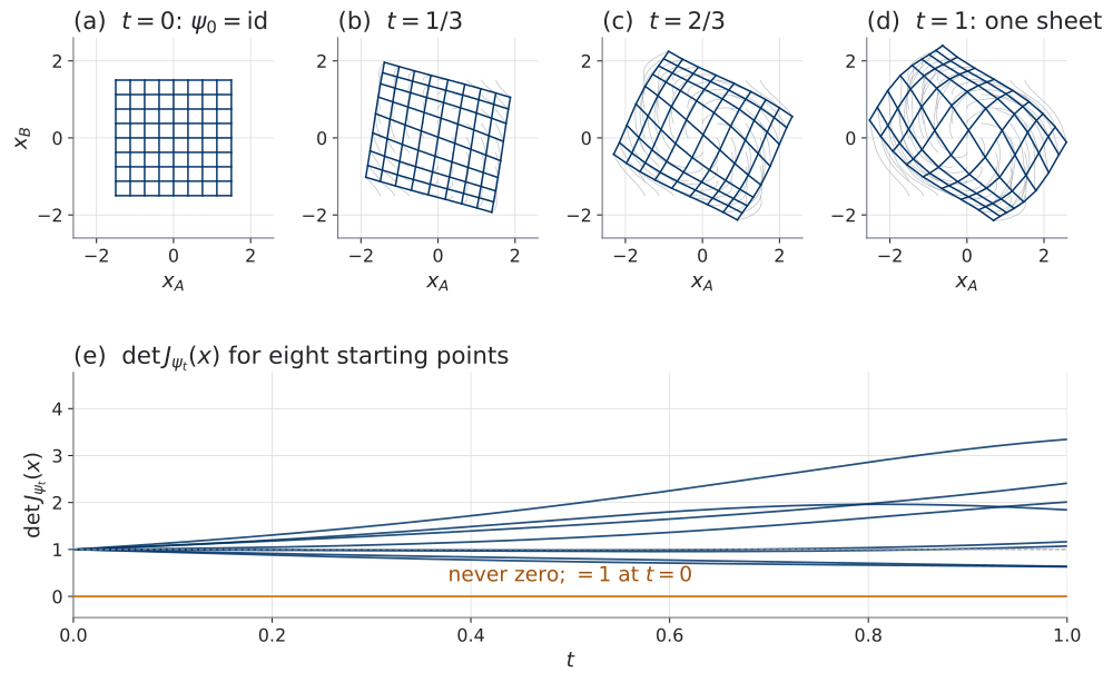
The ODE limit, honestly

The Neural ODE with one depth-independent \(\theta\) is the \(h \to 0\) limit of the Euler stack in which every block evaluates the same \(f_\theta\). It is not the literal continuum limit of a generic ResNet: a ResNet has its own \(\theta_k\) per block, so its natural continuum object carries a depth-dependent path \(t \mapsto \theta(t)\), not a single \(\theta\) (Massaroli et al. 2020, sec. 3).

The ODE limit is a disciplined motivation for the model, not an identity between arbitrary finite ResNets and autonomous-parameter ODEs.

Fourteen to fifteen minutes. Say it in two sentences and move on. Massaroli’s depth-variant models, augmentation and data-control are literature texture: one pointer sentence in the notes, nothing here.

02Well-posedness

What could go wrong

Fifteen to seventeen minutes. (a) Non-uniqueness: x-dot = x^(1/3) from 0. The zero function solves it, and so does every function that waits at 0 until time c and then leaves along ±(2(t-c)/3)^(3/2): eleven drawn, infinitely many exist. The field is continuous and not Lipschitz at 0 — measured slope across zero at separation 1e-9 is 1.6e6. (b) Blow-up: x-dot = x^2 from 1. Smooth field, unique solution 1/(1-t), reaches 20 at t = 0.95 and leaves every bounded set before t = 1. Local existence is not existence on [0, 1]. The theorem excludes exactly these two, one hypothesis each.

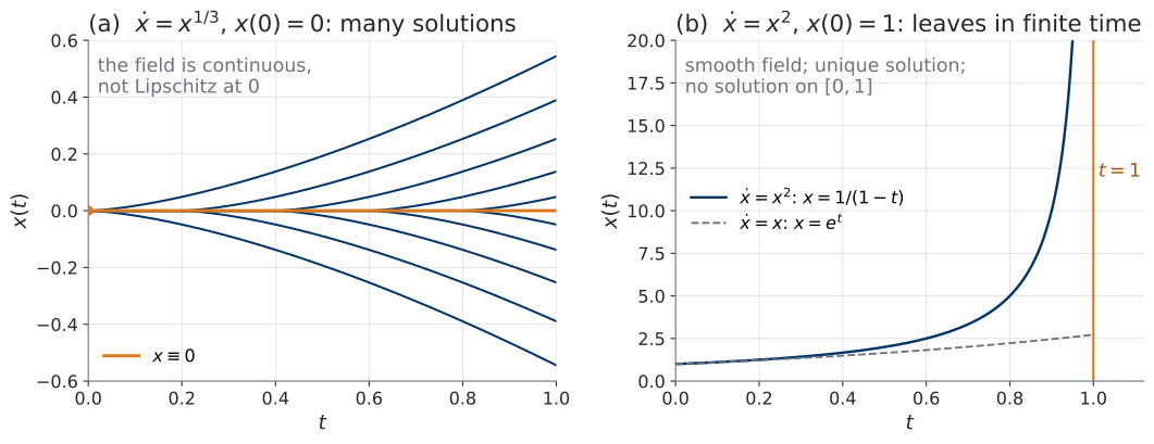
Picard–Lindelöf, at the right strength

Let \(f \colon [0,1] \times \mathbb{R}^{d} \to \mathbb{R}^{d}\) be continuous.

Local. If \(f\) is locally Lipschitz in \(x\), uniformly in \(t\) — on every bounded set \(B\), \(\lVert f(t, x) - f(t, y)\rVert \le L_B \lVert x - y \rVert\) for all \(t\) and \(x, y \in B\) — then for every \(x_0\) there is \(\delta > 0\) and a unique \(C^{1}\) solution on \([0, \delta]\).

Global — the course’s hypothesis. If \(f\) is globally Lipschitz in \(x\), uniformly in \(t\), then for every \(x_0\) the solution exists, is unique and is \(C^{1}\) on all of \([0, 1]\). (Locally Lipschitz + linear growth also suffices.)

Panel (a) failed the Lipschitz hypothesis at \(0\); panel (b) failed linear growth. One hypothesis per failure.

Seventeen to nineteen minutes. State it, name the two failures, and go to the proof engine. Massaroli states the global version in one line and moves on; so do we, except that the students have already written the proof.

The proof engine: PS1.5, on a different space

Write the problem as a fixed-point equation \(x = Tx\) (the map \(T\) is in the table), and let \(L = \operatorname{Lip}(f)\) in \(x\):

	There — PS1.5 (U1.T2)	Here — Picard–Lindelöf
space	\(\mathbb{R}^{d}\), Euclidean norm	\(C([0,1]; \mathbb{R}^{d})\), weighted norm \(\sup_t e^{-2Lt}\lVert x(t)\rVert\)
map	\(T_z(x) = z - g(x)\)	\((Tx)(t) = x_0 + \int_0^{t} f(\tau, x(\tau))\,\mathrm{d}\tau\)
contraction	constant \(\operatorname{Lip}(g) < 1\)	constant \(\tfrac{1}{2}\), bought by the weight \(e^{-2Lt}\)
what buys it	an architectural condition	any finite \(L\) — nothing asked of its size

The line to remember: the residual block needed \(L < 1\); the flow needs \(L < \infty\).

Nineteen to twenty-two minutes. The two-column margin note of the notes, read row by row; the slide keeps four rows, the notes have seven (fixed point: f^{-1}(z) there, the solution on [0, 1] here; uniqueness buys: a bijection there, trajectories that never meet at the same time here). The contraction estimate, on BOARD 2: ||(Tx - Ty)(t)|| <= L ∫_0^t e^{2L tau} d tau · ||x - y||_w <= (1/2) e^{2Lt} ||x - y||_w. Overflow valve: if short on time, read only the “what buys it” row and the last line; the rest is in the notes.

The standing regularity contract for U2

Tier 1 — well-posedness. \(f_\theta\) continuous in \((t, x)\), globally Lipschitz in \(x\) uniformly in \(t\). Enough for existence, uniqueness, invertibility of \(\psi_t\).

Tier 2 — differential identities. In addition, \(f_\theta\) is \(C^{1}\) in \(x\) and in \(\theta\) with continuous partials. Enough for the adjoint (today) and for the divergence identities (U2.T2). Then \(\psi_t\) is \(C^{1}\) in \(x_0\) with invertible Jacobian, and \(t \mapsto J_{\psi_t}(x_0)\) is continuous.

Course models use tanh / softplus and satisfy both tiers. ReLU is Lipschitz and not \(C^{1}\): Tier 1 only. The two roles are never conflated in this unit.

Twenty-two to twenty-three minutes. Two tiers, one sentence each, and the ReLU remark. Every statement of the unit names its tier.

Invertibility by well-posedness, not for free

Under Tier 1, for \(t_0 < t_1\) the map \(\psi_{t_0 \to t_1}\) is a bijection of \(\mathbb{R}^{d}\), and its inverse is obtained by integrating the same equation backward in time from \(t_1\) to \(t_0\); both directions are continuous (Grönwall), so it is a homeomorphism. Under Tier 2 it is a diffeomorphism.

Proof in one line each. Injective: two solutions meeting at time \(t_1\) coincide (uniqueness, run backward). Surjective: solve backward from any \(y\) at \(t_1\). Continuous: Grönwall bounds the spread of two solutions by \(e^{L}\) times their initial spread, in both directions.

Twenty-three to twenty-four minutes. Injective, surjective, continuous: one line each on BOARD 2.

The inverse: words, and cost

• Words. “The flow of \(-f\)” is right only after time reversal: \(y(\tau) = x(t_1 - \tau)\) solves \(\dot y = -f(t_1 - \tau, y)\), a different non-autonomous field. “Integrate the same equation backward” is always right.
• Cost. No coupling pattern, no triangular Jacobian, no contraction per block — structurally automatic. And not free: the inverse is an ODE solve, priced in NFE (the number of times the solver evaluates \(f_\theta\)). Both directions of the map pay in that currency.

Twenty-four to twenty-five minutes. On BOARD 1, the left board: write “inverse: ODE solve / NFE” in the Neural ODE row that is about to appear. Do not write “flow of -f” on the board; say why.

What a regular flow cannot do in one dimension

Twenty-five to twenty-six minutes. (a) Eleven trajectories of a regular 1-D field: no two cross; the smallest gap over the whole interval is 0.12. Why: if two met at some time, uniqueness run backward would make them the same trajectory. (b) The measured time-1 map is increasing (slopes 0.18 to 1.64); the reflection x -> -x is decreasing, so it is not a 1-D flow map. This is Massaroli’s “crossing trajectories” problem, read as order preservation and nothing more. (c) The plane: f = pi R x carries an off-centre grid to its image under -I along half-circles; psi_1 = -I to 3e-13, det = 1. What is impossible on the line is a rotation on the plane.

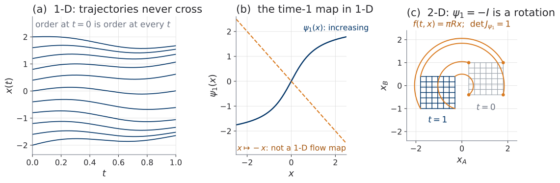
What a regular flow map cannot be

Let \(f\) satisfy Tier 1 and \(\psi_t\) be its flow.

(i) \(d = 1\): order is preserved. \(x_0 < y_0 \Rightarrow \psi_t(x_0) < \psi_t(y_0)\) for all \(t\). So \(\psi_1\) is strictly increasing, and \(x \mapsto -x\) is not a 1-D regular flow map.

(ii) Any \(d\): orientation is preserved. Under Tier 2, \(\det J_{\psi_t}(x) > 0\) for all \(x, t\): continuous in \(t\), equal to \(1\) at \(t = 0\), never zero. So \(x \mapsto -x\) (determinant \((-1)^{d}\)) is not a regular flow map in odd \(d\); in \(d = 2\) it is a rotation.

(iii) Orientation is necessary, not a characterization; finer claims are dimension-specific and not made here.

Twenty-six to twenty-eight minutes. Proof of (ii) in three words on BOARD 2: continuous, one at zero, never zero, therefore positive. “Never zero” is because psi_t is a diffeomorphism.

What this restriction is not

• It is not U1.T2’s topology-obstruction-argument. That one is about supports under a homeomorphism — still true here, unchanged, because \(\psi_1\) is a homeomorphism. Today’s is about which maps arise as flows at all.
• U3 cites the two side by side, never one inside the other.

U3 changes what density path we prescribe, but any regular ODE flow map is still a regular flow map. Hold the thought.

Twenty-eight to twenty-nine minutes. Say the separation sentence about U1’s artifact once. Then the gray sentence: U3 changes what density path we prescribe, but any regular ODE flow map is still a regular flow map — hold the thought.

The two costs, version 2, annotated

Family	Density	Sampling	Trick, and its price
NICE / RealNVP	exact, triangular	direct	coupling; depth
Glow	exact	direct	mixing, multi-scale
MAF	parallel	sequential	AR, data side
IAF	sequential	parallel	AR, source side
Residual flow	direct; series log-det	iterative	contraction, traces
Neural ODE	inverse: ODE solve / NFE; \(\log\lvert\det J\rvert\) ???	ODE solve / NFE	no inverse layer; Lipschitz field

Twenty-nine to thirty minutes. This is BOARD 1 as it now stands. Read the row aloud in full: inverse resolved with no layer to design, only a Lipschitz field; runtime an ODE solve in both directions, priced in NFE; log-determinant open. Circle the ??? at the close, not now. Not version 3 — the U1 cells are untouched.

03The adjoint method

The setup, and one letter

Fix \(x_0\); \(x\) solves \(\dot x = f_\theta(t, x)\) under Tier 2; the loss reads the endpoint:

\[ \ell(\theta) = L\big(x(1)\big), \qquad L \in C^{1}. \qquad\text{Wanted: } \frac{\mathrm{d}\ell}{\mathrm{d}\theta} \in \mathbb{R}^{1 \times p}. \]

• Cotangents — the row vectors that multiply Jacobians from the left in reverse mode — are rows: the adjoint state is \(a^{\top}(t) \in \mathbb{R}^{1 \times d}\).
• Goal: \(\mathrm{d}\ell/\mathrm{d}\theta\) without storing every solver-internal state.
• One letter. Today \(\mathcal{L}\) is not a loss. It is the perturbed functional of the derivation; the loss is \(\ell\). They agree in value along trajectories — that is the trick — and are different functions. The roman \(L\) here is the loss function, not the Lipschitz constant of the well-posedness block.

Thirty to thirty-one minutes. Erase BOARD 2. Draw three empty rectangles on it, labelled G1, G2, G3, before writing anything else: the derivation is going to be written around them, and they are PS2.1. Say the letter sentence once.

Step 0 — the discrete ancestor

For \(F = f_K \circ \cdots \circ f_1\) (\(K\) maps), \(x^{k} = f_k(x^{k-1})\), \(x^{0} = x\), and a cotangent \(v^{\top}\) on the output: \[ \begin{aligned} v_K^{\top} &= v^{\top}, \qquad v_{k-1}^{\top} = v_k^{\top} J_{f_k}(x^{k-1}) \;\; (k = K, \dots, 1), \\ v_0^{\top} &= v^{\top} J_F(x). \end{aligned} \] Each step is a vector–Jacobian product (VJP): about one \(f_k\)-evaluation, no Jacobian formed.

Backprop pushes a cotangent backward through composed maps. The adjoint pushes a cotangent backward through continuously composed maps.

Thirty-one to thirty-four minutes. Two lines, one tag: “proved in the bootcamp; one-line context”. PGMAT hears the callback to U0.T1’s Proposition 1; PESC sees the whole statement.

Step 0, continued — the layers as Euler steps

Let the layers be Euler steps, \(f_k(x) = x + h f(t_{k-1}, x)\), so \(J_{f_k} = I + h\,\partial f/\partial x\): \[ v_{k-1}^{\top} = v_k^{\top} + h\, v_k^{\top}\, \frac{\partial f}{\partial x}(t_{k-1}, x_{k-1}) \quad\xrightarrow{\;h \to 0\;}\quad \dot a^{\top} = -\,a^{\top}\, \frac{\partial f}{\partial x}. \]

The adjoint state is the running VJP. Whether the recursion is exactly the discrete adjoint is PS2.1(g).

Thirty-four to thirty-six minutes. The arrow is a heuristic, said as one — the proof that follows makes no limit.

Step 1 — the perturbed functional (G2, first half)

Fix \(\theta_0\). For any \(C^{1}\) function \(a \colon [0,1] \to \mathbb{R}^{d}\), chosen once as a function of \(t\) alone:

\[ \mathcal{L}(\theta) = \ell(\theta) - \int_0^{1} a^{\top}(t)\,\big[\dot x(t) - f_\theta\big(t, x(t)\big)\big]\,\mathrm{d}t . \]

The bracket is identically zero, because \(x\) solves the equation — for every \(\theta\).

So \(\mathcal{L} = \ell\) as functions of \(\theta\), and \(\dfrac{\mathrm{d}\mathcal{L}}{\mathrm{d}\theta} = \dfrac{\mathrm{d}\ell}{\mathrm{d}\theta}\), whatever \(a\) is. \(a\) is free. We will spend it.

Thirty-six to thirty-eight minutes. This is G2, first half: why we are allowed to choose a at all. Write only the label “G2: why is a free?” in the second box, and the claim, then continue.

Step 2 — integration by parts (G1)

\[ \int_0^{1} a^{\top}\dot x\,\mathrm{d}t = a^{\top}(1)\,x(1) - a^{\top}(0)\,x(0) - \int_0^{1} \dot a^{\top} x\,\mathrm{d}t . \]

Stated, not performed: boundary terms plus a sign flip. Check it — that is PS2.1(b). With it, \[ \mathcal{L}(\theta) = L\big(x(1)\big) - a^{\top}(1)\,x(1) + a^{\top}(0)\,x_0 + \int_0^{1} \Big[\dot a^{\top} x + a^{\top} f_\theta(t, x)\Big]\mathrm{d}t . \]

Thirty-eight to forty minutes. G1 is the first empty box: write “G1: integrate by parts” and the result, not the steps. Move on.

Step 3 — differentiate, and collect the sensitivity

Write \(S(t) = \mathrm{d}x(t)/\mathrm{d}\theta \in \mathbb{R}^{d \times p}\) (exists and is continuous under Tier 2), with \(S(0) = 0\) because \(x_0\) does not depend on \(\theta\). Let \(A = \partial f_\theta/\partial x\), \(B = \partial f_\theta/\partial\theta\), both along the trajectory.

\[ \begin{aligned} \frac{\mathrm{d}\mathcal{L}}{\mathrm{d}\theta} &= \underbrace{\Big[\frac{\partial L}{\partial x}\big(x(1)\big) - a^{\top}(1)\Big] S(1)} _{\text{multiplies the unknown } S(1)} + \underbrace{\int_0^{1} \Big[\dot a^{\top} + a^{\top} A\Big] S\,\mathrm{d}t}_{\text{multiplies the unknown } S(t)} \\ &\quad + \underbrace{\int_0^{1} a^{\top} B\,\mathrm{d}t}_{\text{no sensitivity at all}} \end{aligned} \]

Forty to forty-eight minutes. The slowest slide of the session, and the one genuinely error-prone bookkeeping step: done slowly, once, clean. Say that the term a^T(0) S(0) vanished, and why. On BOARD 2, differentiate the four terms of the previous slide one by one and sort them into the three groups; the students must see it done clean once. Say where S(0) = 0 came from.

Step 4 — spend the free choice (G2)

Why are we allowed to choose \(a\)? Because Step 1 holds for every fixed \(a\). So choose the one that annihilates both sensitivity groups:

\[ \dot a^{\top}(t) = -\,a^{\top}(t)\, \frac{\partial f_\theta}{\partial x}\big(t, x(t)\big), \qquad a^{\top}(1) = \frac{\partial L}{\partial x}\big(x(1)\big). \]

A linear final-value problem, solved backward from \(t = 1\); it exists, is unique and is \(C^{1}\) by Picard–Lindelöf (continuous coefficient matrix). With this \(a\), both unknown groups vanish whatever \(S\) is.

A free choice, spent wisely — the same proof taste as the projection Lemma’s session, and no formal connection claimed.

Forty-eight to fifty-two minutes. G2, second half: write “G2: why may we choose a? — articulate it” in the box; the answer they must write in PS2.1(a)/(d) is that the bracket is identically zero so L-script equals l for every a. Echo the Lemma session’s rhetoric, and say explicitly that no formal connection is claimed.

What survives: the adjoint sensitivity theorem

Under Tier 2, with \(x_0\) independent of \(\theta\) and \(\ell = L(x(1))\), \(L \in C^{1}\): \[ \begin{aligned} \frac{\mathrm{d}\ell}{\mathrm{d}\theta} &= \int_0^{1} a^{\top}(t)\, \frac{\partial f_\theta}{\partial \theta}\big(t, x(t)\big)\,\mathrm{d}t, \\ \dot a^{\top} &= -\,a^{\top}\,\frac{\partial f_\theta}{\partial x}, \qquad a^{\top}(1) = \frac{\partial L}{\partial x}\big(x(1)\big). \end{aligned} \] Moreover \(a^{\top}(t) = \mathrm{d}\ell/\mathrm{d}x(t)\): the sensitivity of the loss to the state at time \(t\) — the running VJP (Chen et al. 2018, App. B).

Named, boxed, and on the right board for the rest of the session. The full gap-free derivation is Box U2.T1-3 of the notes; the gaps are PS2.1.

Fifty-two to fifty-four minutes. BOARD 3 (right, persistent): the theorem, boxed, under the log-det question. It stays there. Name it out loud: the adjoint sensitivity theorem.

Implementation: the augmented backward solve (G3)

Add one state, the parameter adjoint \(a_\theta(t) \in \mathbb{R}^{p}\): \[ \dot a_\theta^{\top} = -\,a^{\top}\,\frac{\partial f_\theta}{\partial\theta}\big(t, x(t)\big), \qquad a_\theta(1) = 0 . \]

Recipe (Chen et al. 2018, Alg. 1): solve \((x, a, a_\theta)\), dimension \(2d + p\), backward from \(t = 1\) to \(0\), from \(\big(x(1),\; \partial L/\partial x(x(1))^{\top},\; 0\big)\) with dynamics \(\big(f_\theta,\; -A^{\top} a,\; -B^{\top} a\big)\); read \[ \frac{\mathrm{d}\ell}{\mathrm{d}\theta} = a_\theta(0)^{\top}. \]

\(x(t)\) is reconstructed backward beside \(a\), not stored. Why \(a_\theta(0)\) equals the boxed integral is PS2.1(e).

Fifty-four to fifty-eight minutes. G3: the third box gets “G3: why does a_theta(0) compute the integral?” — stated as a recipe, derived by them. Each RHS term a^T df/dx and a^T df/dtheta is a VJP: about one f-evaluation each, no Jacobian formed, so a backward RHS call costs a small constant multiple of a forward one. The backward pass has its own NFE bill.

The two passes, on one time axis

Fifty-eight to fifty-nine minutes. Forward lane: x_0 to x(1) to the loss. Backward lane: a from its terminal value down to t = 0. Third lane: a_theta accumulated beside a, read at t = 0. Dashed: the state reconstructed, not stored — that is both the memory saving and the numerical asterisk of the strategies block.

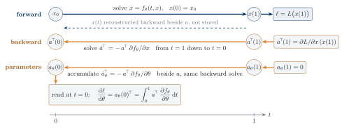
Worked example: the scalar field, differentiated twice

\(f_\theta(t, x) = -\theta x\) on \(\mathbb{R}\), \(x(0) = x_0\), \(L(x) = \tfrac{1}{2} x^{2}\).

Directly. \(x(1) = x_0 e^{-\theta}\), so \(\ell = \tfrac{1}{2} x_0^{2} e^{-2\theta}\) and \(\mathrm{d}\ell/\mathrm{d}\theta = -x_0^{2} e^{-2\theta}\).

By the adjoint. \(\partial f/\partial x = -\theta\): \(\dot a = \theta a\), \(a(1) = x_0 e^{-\theta}\), so \(a(t) = x_0 e^{\theta(t-2)}\). And \(\partial f/\partial\theta = -x_0 e^{-\theta t}\): \[ \int_0^{1} a\,\frac{\partial f}{\partial\theta}\,\mathrm{d}t = -x_0^{2}\int_0^{1} e^{\theta(t-2)} e^{-\theta t}\,\mathrm{d}t = -x_0^{2} e^{-2\theta}. \quad\checkmark \]

And \(a(t) = \mathrm{d}\ell/\mathrm{d}x(t)\): \(\ell = \tfrac{1}{2} x(t)^{2} e^{-2\theta(1-t)}\) has derivative \(x(t) e^{-2\theta(1-t)} = x_0 e^{\theta(t-2)}\). The adjoint is the running sensitivity.

Fifty-nine to sixty-one minutes. The running example, closed. Two computations agree; the third line is the interpretation checked.

The punchline, said aloud

For a fixed number of requested output times, the continuous adjoint stores \(x(1)\), \(a\), \(a_\theta\) and the solver’s current step: \(O(1)\) state with respect to the number of solver steps. Direct backprop stores every intermediate state the solver produced.

The price, both halves:

1. another numerical solve, of dimension \(2d + p\), with its own NFE;
2. an optimize-then-discretize gradient: an approximation of the exact solution’s gradient, not the exact gradient of the discretized forward map.

Sixty-one to sixty-three minutes. Two minutes at most. The strategies block reads the price slowly.

Bonus: the generalized adjoint (no proof)

For \(\ell = L(x(1)) + \int_0^{1} l(t, x(t), \theta)\,\mathrm{d}t\), \(l \in C^{1}\): \[ \dot a^{\top} = -\,a^{\top}\frac{\partial f_\theta}{\partial x} - \frac{\partial l}{\partial x}, \qquad \frac{\mathrm{d}\ell}{\mathrm{d}\theta} = \int_0^{1}\Big[a^{\top}\frac{\partial f_\theta}{\partial\theta} + \frac{\partial l}{\partial\theta}\Big]\mathrm{d}t . \]

Proposition 1 of Massaroli et al. (2020) proves the case \(l = l(t, x)\), with no explicit \(\theta\); the direct \(\partial l/\partial\theta\) term is what appears when the integrand depends on the parameters — a regularizer on the learned field itself (U2.T2 meets one). “Integral loss” is not merely an extra state derivative.

Sixty-three to sixty-five minutes. One slide, no proof. Say why the second term matters: RNODE-style regularizers depend on the field, hence on theta, explicitly.

04Backprop through the solver, or the adjoint

The two strategies

	Memory	Compute	Correctness
Direct backprop through the solver (discretize \(\to\) optimize)	every stored solver state; grows with the steps	forward solve + one reverse sweep of VJPs	for a fixed-step solver: the exact gradient of the executed discrete map
Continuous adjoint (optimize \(\to\) discretize)	\(O(1)\) in the steps, at a fixed number of requested output times	a second solve, dimension \(2d + p\), each RHS call an \(f_\theta\) plus VJPs	an approximation of the exact-solution gradient; two discretizations; reconstruction can drift

Sixty-five to sixty-eight minutes. Read the table row by row. The correctness column is where they differ in kind; next slide.

Correctness, read slowly

Discretize, then optimize. A fixed-step solver computes a specific composition of arithmetic; autodiff differentiates that. Exact for the function the computer evaluated — not for the exact solution. For an adaptive solver the step controller’s decisions are treated as constants: a statement about the executed trace, locally valid, not globally smooth.

Optimize, then discretize. Derive the gradient of the exact solution’s loss (the theorem), then discretize the adjoint equation. Close to the true gradient when both solves are accurate — and not the gradient of anything the forward solver computed.

Neither is “the correct one”: exact for the wrong function, or approximate for the right one. Which is better is empirical — U2.L1 asks it with a table.

Sixty-eight to seventy-one minutes. The distinction returns in U3 for solver error in samples; say so in one sentence. Same taxonomy, different object.

The asterisk under invertibility

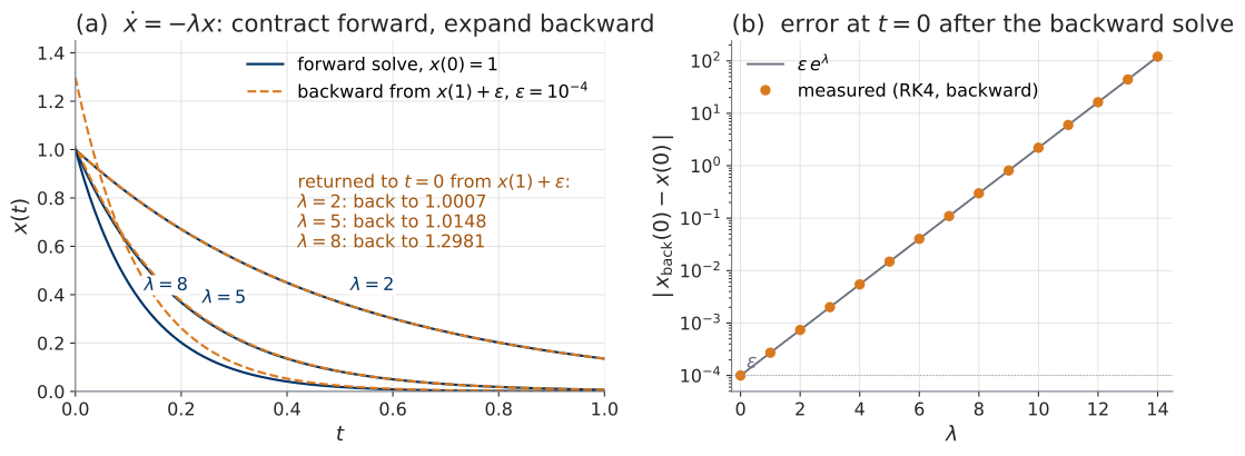
RK4 is the fourth-order Runge–Kutta solver; \(\varepsilon = 10^{-4}\) is injected at \(t = 1\).

Seventy-one to seventy-four minutes. One mechanism on one field with a known answer: x-dot = -lambda x contracts forward by e^(-lambda), so backward it expands by e^(lambda). (a) A perturbation of 1e-4 at t = 1 returns to 1.0007, 1.0148 and 1.2981 instead of 1, for lambda 2, 5, 8. (b) Measured error at t = 0 against epsilon e^lambda: on the line to 3e-10 relative, over lambda from 0 to 14. Without the perturbation the backward solve returns to 1 to 3e-12 even at lambda 14 — the drift is the amplified perturbation, not the solver. It measures no gradient and says nothing about a trained model: that is U2.L1’s table. It says why the table has to exist.

Mitigations, named and not oversold

• Tighter tolerances on the backward solve — costs NFE.
• Direct backpropagation when the problem is small enough to store.
• Checkpointing / hybrid schemes: store a few forward states, reconstruct only between them — bounded reconstruction length, in systems that support it.

Libraries, stated carefully: torchdiffeq (Chen 2018) offers the continuous adjoint as odeint_adjoint. Diffrax (Kidger 2021) makes recursive checkpointing its default and offers the continuous adjoint as a contrast — the contrast U2.L1 uses.

None of these is a theorem. Each is an engineering choice with a bill. Beyond the course: (Kidger 2022, sec. 5.1).

Seventy-four to seventy-six minutes. Do not claim a torchdiffeq “store the whole trajectory” option; there is none to claim. Diffrax’s recursive checkpointing appears in the lab as the modern counterpoint.

The plot you will make

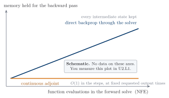
In U2.L1 you produce the memory-against-NFE plot yourselves, on a small classifier where nothing hurts yet, and compare it to this schematic. The data is yours to make.

Seventy-six to eighty minutes. Hand-drawn axes, no data, by decision. The lab installs the gauges — NFE counter, memory probe, gradient-fidelity check — so that U2.L2 can point them at a generative model.

05Close

PS2.1, assigned at the board (1 of 2)

Setting: \(\dot x = f_\theta(t, x)\), \(x(0) = x_0\), \(\ell = L(x(1))\), \(f_\theta\) continuously differentiable, Lipschitz in \(x\).

• (a) Define the perturbed functional \(\mathcal{L}\) with multiplier \(a(t)\) and justify \(\mathrm{d}\ell/\mathrm{d}\theta = \mathrm{d}\mathcal{L}/\mathrm{d}\theta\) for every choice of \(a\). [= G2, part 1]
• (b) Carry out the integration by parts, tracking boundary terms at \(t = 0\) and \(t = 1\) explicitly. [= G1]
• (c) Differentiate \(\mathcal{L}\) w.r.t. \(\theta\) and collect all terms containing \(\mathrm{d}x/\mathrm{d}\theta\). Explain why \(\mathrm{d}x(0)/\mathrm{d}\theta = 0\).
• (d) Exhibit the choice of final-value problem for \(a(t)\) that annihilates every \(\mathrm{d}x/\mathrm{d}\theta\) term; conclude the adjoint sensitivity theorem. [= G2, part 2]

Eighty to eighty-four minutes. BOARD 3: list (a)–(d) beside the boxed theorem, each with its G-number.

PS2.1, assigned at the board (2 of 2)

• (e) Derive the augmented-state implementation: show that \(a_\theta(0)\) as defined in lecture equals the boxed integral. [= G3]
• (f) Bonus. Extend (a)–(d) to \(\ell = L(x(1)) + \int_0^{1} l(t, x(t), \theta)\,\mathrm{d}t\). Recover both the \(-\partial l/\partial x\) term in the adjoint ODE and the direct \(\partial l/\partial\theta\) contribution to \(\mathrm{d}\ell/\mathrm{d}\theta\) (Massaroli et al. 2020, Prop. 1); attached PDF only after attempting.
• (g) Bonus. Euler-discretize the forward ODE with step \(h\) and show the adjoint recursion at the discrete points is exactly reverse-mode autodiff through the unrolled steps (the VJP identity from lecture). Conclude in one sentence in what precise sense “the adjoint is backprop’s continuum limit.”

Eighty-four to eighty-six minutes. BOARD 3: (e)–(g) under (a)–(d). The three empty boxes on BOARD 2 and the list on BOARD 3 are visible at the same time: the visual of three gaps inside an otherwise complete derivation IS the assignment. Part (g)’s sentence is the session’s thesis; it is not in the notes, and it is not in the key until PS2 solutions release.

The board at the close

Left board	Right board	Top right
the two costs, v2 annotated: inverse resolved, runtime ODE solve / NFE, log-determinant ??? — circled	the adjoint sensitivity theorem, boxed; PS2.1 (a)–(g) with their G-numbers	What does \(\log\lvert\det J\rvert\) become in continuous time? — not erased

We can now build continuous-depth invertible maps and differentiate them without storing every solver step. What we cannot yet do is account for their density change cheaply. The lab measures the numerical bill; U2.T2 finds out what \(\log\lvert\det J\rvert\) became.

Eighty-six to eighty-nine minutes. Circle the ??? on BOARD 1 now. Read the last sentence verbatim, and out.

Reading the board

On the board	Status
Residual steps \(\to\) an ODE	Made precise, with the honest caveat
Existence, uniqueness	Yes, under a Lipschitz field — two tiers recorded
Invertibility	Structurally automatic; computationally an ODE solve — orientation preserved
Differentiating through a solver	The adjoint sensitivity theorem — gaps G1–G3 = PS2.1
\(\log\lvert\det J\rvert\) in continuous time	Open. U2.T2

Next session: the lab (U2.L1), solvers and adjoints in practice. The theory session after it (U2.T2) opens on the circled cell.

Eighty-nine to ninety minutes. Read the five rows and out.

References

Chen, Ricky T. Q. 2018. “torchdiffeq: ODE Solvers and Adjoint Sensitivity Analysis in PyTorch.” https://github.com/rtqichen/torchdiffeq.

Chen, Ricky T. Q., Yulia Rubanova, Jesse Bettencourt, and David Duvenaud. 2018. “Neural Ordinary Differential Equations.” In Advances in Neural Information Processing Systems. https://arxiv.org/abs/1806.07366.

Kidger, Patrick. 2021. “Diffrax: Numerical Differential Equation Solvers in JAX.” https://github.com/patrick-kidger/diffrax.

———. 2022. “On Neural Differential Equations.” PhD thesis, University of Oxford. https://arxiv.org/abs/2202.02435.

Massaroli, Stefano, Michael Poli, Jinkyoo Park, Atsushi Yamashita, and Hajime Asama. 2020. “Dissecting Neural ODEs.” In Advances in Neural Information Processing Systems. https://arxiv.org/abs/2002.08071.