U1.L1 — Coupling Flows on 2D Toys
Session U1.L1 · date: see calendar-map
How to read this page. This is the first lab of the joint phase, and the first time in this course that a generative model is written from nothing and trained. The previous session (U1.T1) proved that a coupling layer has a cheap inverse and a log-determinant that is a sum read off one forward pass. Today you write that layer, stack it, check the sum against an automatic differentiation Jacobian that owes nothing to your derivation, train the stack by exact maximum likelihood on two-dimensional toy data, and look at what it learned. Then you check it against a library, and read the library’s source with your own code beside it.
These notes are the written record of the lab; the executable part is the notebook labs/lab-u1l1.ipynb (the instructor releases its solutions, lab-u1l1-solutions.ipynb). The page is self-contained on purpose. It depends on U1.T1 and on nothing else: where a bootcamp artifact is named, the thing it names is written out here in full, and you do not need to have attended the bootcamp.
Two references are optional: (Dinh, Sohl-Dickstein, and Bengio 2017) §3.2–3.3 is the layer you implement, and §3.5 is how its copies are combined; (Papamakarios et al. 2021) §3.1.2 is the same layer in a survey’s notation. (Rozet et al. 2022) is the library of §5.
Every number on this page was measured. The runs behind the figures are in scripts/python/fig_u1_l1_coupling_flows.py, seeded, on CPU, and the values are recorded in scripts/python/_outputs/u1l1_coupling_flows.json. Re-running the script reproduces every one of them to the digit; the wall-clock times are the only values that move.
- A bijection you wrote:
AffineCoupling, and aFlowthat stacks it, each with an inverse and a log-determinant in both directions. - Exact density evaluation:
Flow.log_prob, which is U1.T1’s change-of-variables theorem as code, and the loss of §3. - An independent Jacobian witness: a per-example, float64, automatic differentiation Jacobian, against which your analytic log-determinant is checked before and after training.
A fourth thing is deliberately not on the list: an explanation of what the last figure shows in the checkerboard’s gaps. That is U1.T2’s opening.
0 · Orientation and handover
Block 0 of the lab, 10 minutes. Reused in: every later joint lab, as the pattern.
Given code, and the parity rule
Three modules under common/ arrive as given code. Two of them were built in bootcamp sessions; that is provenance, not a prerequisite. What the lab uses of each is its contract, and the contracts are all written here.
| Module | Built in | What this lab uses |
|---|---|---|
common/train.py |
U0.L1, extended in U0.L2 | set_seed(seed); Trainer(model, opt, loss_fn, device, ckpt_dir, log_every, *, sched, tracker, config) with .fit(train_loader, val_loader, epochs) |
common/toy2d.py |
today, §1 | the three frozen generators and two picture helpers |
common/coupling.py |
today, the reference you rebuild | imported at the end, to cross-check your own module |
The Trainer runs the five-step loop, forward → loss → zero_grad → backward → step, then sched.step() per step; evaluates on the validation loader under no_grad every epoch; writes last.pt every epoch and best.pt when the validation loss improves; and logs to a CSV file in the run directory. Its interface was frozen for classifiers, which is why it takes (x, y) batches and reports an accuracy. A flow has no labels, so y is a placeholder and the accuracy reads nan. That is an interface being preserved, not a defect.
This lab is the first instance of a rule that binds every joint session (L1 §2): a joint session may consume bootcamp-built artifacts as given code, with a contract-level description, and may never require having attended the bootcamp. The provenance of a module may be named, as in Table 1. The content of the session must not depend on it. Every later joint lab follows the same pattern as this block.
Where the curves go
The course logs to MLflow, deployed locally: a SQLite file next to the notebook, sqlite:///mlflow.db, plus a mlartifacts/ directory, both gitignored. The store is local because an offline teaching bundle must stand alone; a run directory can be zipped and handed to someone with no server in between. It is not a recommendation of any backend for production. (The mlruns/ file-store layout of older tutorials is deprecated in MLflow 3.15, which is why the course settled on SQLite in U0.L2.) After training, mlflow ui --backend-store-uri sqlite:///mlflow.db shows the curves.
One departure from the bootcamp wiring, with its reason. The Trainer can log to MLflow per step, and for an image model that is the right cadence. Here a step is a 256-point batch through a network of 26,508 parameters, and it runs in under a millisecond, while one SQLite write costs a few milliseconds. Measured: per-step tracking turned a 14 s training into a 48 s one. So the loop runs without the tracker, its CSV log and checkpoints still go to runs/, and the two NLL curves (the negative log-likelihood, the loss of §3, on the training and the validation sets) are logged per epoch, after the loop, with the resolved configuration and the tags. The run directory stands alone either way, which is the rule that matters.
The sanity ritual, and today’s sibling of it
The course-wide ritual, performed in every lab: after writing anything that claims to be a derivative, compare it with finite differences, in float64, along one fixed unit direction \(v\),
\[ v^{\top}\nabla_\theta L \;\approx\; \frac{L(\theta+\varepsilon v)-L(\theta-\varepsilon v)}{2\varepsilon}, \qquad \lVert v \rVert = 1 , \]
accepted under the mixed tolerance \(|d_{\mathrm{AD}} - d_{\mathrm{FD}}| \le \texttt{atol} + \texttt{rtol}\cdot\max(|d_{\mathrm{AD}}|, |d_{\mathrm{FD}}|)\). Two extra forward evaluations, whatever the parameter count. The notebook runs it once on a scalar toy so that the shape is fresh.
Today’s check is a sibling. The object under suspicion is not a gradient but a log-determinant. You will compute \(\log|\det J_\psi|\) analytically, as a sum of scales, and compare it with a Jacobian that automatic differentiation assembles independently, one example at a time, in float64. Same discipline, same mixed tolerance, and the same rule that a check which cannot fail has verified nothing (§2).
1 · toy2d: the datasets, frozen today
Block 1, 8 minutes. Produces the artifact toy2d-datasets. Reused in: U2.L1, U2.L2, U3.L1, U3.L3, and the U6 seminar notebooks.
common/toy2d.py is infrastructure, not an exercise: it is distributed complete and frozen from today. The reason is a contract with two later sessions. U2.L2 and U3.L1 train other models on exactly these points and compare them with what you build today, and the comparison means something only if the generator and the seeds are the same. So downstream sessions import this module by name and never redefine a generator.
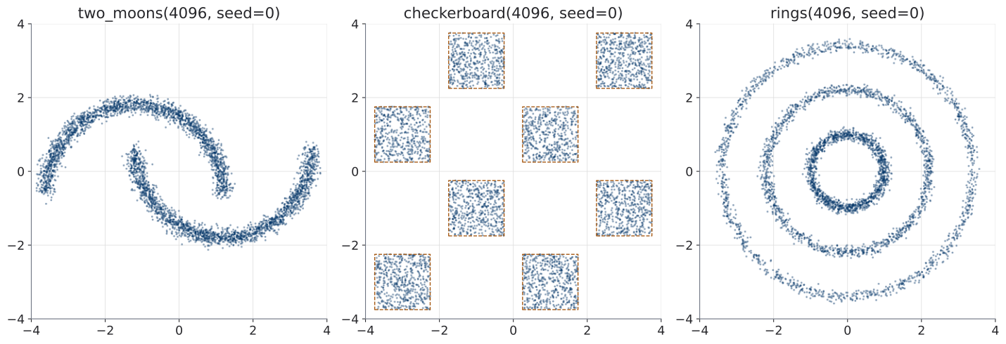
seed=0, 4096 points each, on the default extent \([-4,4]^2\). Left: two interleaving half-circles with isotropic Gaussian jitter. Middle: the gapped checkerboard, eight separated squares of side \(1.5\) (outlined); there is no jitter and no mass outside the squares. Right: three concentric rings with a thin radial profile.
common/toy2d.py

two_moons(n, seed)     -> Tensor (n, 2), float32
checkerboard(n, seed)  -> Tensor (n, 2), float32
rings(n, seed)         -> Tensor (n, 2), float32
EXTENT = (-4.0, 4.0)   # default plotting extent, both axes

density_heatmap(log_prob_fn, extent=EXTENT, n=200, ax=None)
    -> (xs, ys, logp)
warped_grid(generative_fn, extent=EXTENT, ax=None, ...)
-> lines- Pure, seeded functions. Each generator owns a
numpy.random.default_rng(seed); nothing reads or advances a global stream. Sameseed, same pinned environment (environment.yml), same tensor, bit for bit. - Float32 outputs, shape
(n, 2). The flows train in float32; the checks promote to float64 themselves. - The checkerboard has literal zero-density gaps. It is an equal-weight mixture of eight separated squares of side \(1.5\), centred in the black cells of a \(4 \times 4\) board on \([-4,4]^2\), with no Gaussian jitter. Two same-colour squares are diagonal neighbours whose nearest corners are \(0.5\sqrt{2} \approx 0.71\) apart; the white cells carry no mass at all. The support of \(q\) is a union of eight disjoint closed squares, and its density is exactly \(1/18\) on that support.
Property 3 is the one to read twice. It is a mathematical statement about the support of the data distribution, and it is there because U1.T2 makes a statement about literal support and needs a witness. The figure script checks it the only way a support claim can be checked by sampling: of \(100{,}000\) checkerboard points, \(0\) fall outside the eight squares. The notebook’s Checkpoint 1 executes the whole contract: bit-identical across calls, seed-sensitive, and the same \(100{,}000\)-point support test. Today you only observe what a fitted density does in the gaps.
The two picture helpers are the visualization contract of the unit. density_heatmap evaluates a log_prob function on an \(n \times n\) grid over the extent, in chunks, and draws \(e^{\log p}\) with imshow. (Not with a Gouraud-shaded mesh, whose thousands of gradients render differently in a browser and in a PDF; the repository’s invariants gate refuses that signature.) warped_grid pushes a regular grid of the source space, \([-3, 3]^2\) in the source coordinates, through the generative map and draws the image on the data extent. It is the visual twin of U1.T1’s local-volume picture: a cell that comes out large is a place where the density was divided by a large \(|\det J|\).
U2.L2 and U3.L1 draw two_moons(4096, 0) and compare a solver-trained model and a simulation-free one against the model you train today, on the same points. The gapped checkerboard returns in U1.T2 as the controlled witness of its opening result, and in U3.L1 as the dataset on which that result is revisited.
2 · An affine coupling layer, from scratch
Block 2, 20 minutes. Produces the artifact coupling-layer-scratch. Reused in: PS1.4 (verification), U1.L2 (the affine algebra), every flow lab.
Reference for this section: (Dinh, Sohl-Dickstein, and Bengio 2017) §3.2 (the layer), §3.3 (its properties) and §3.5 (alternating the halves across layers); U1.T1 §5 for the derivation.
The layer, in the generative direction
The course’s generative map is \(\psi \colon z \to x\), and every layer is written in that direction. Split the coordinates into an untouched half \(x_A\), which the conditioner reads, and a moved half \(x_B\):
\[ \begin{aligned} \text{forward:}\quad & y_A = x_A, \qquad y_B = x_B \odot e^{s_\theta(x_A)} + t_\theta(x_A), \\ & \log\big|\det J_\psi(x)\big| = \textstyle\sum_j s_\theta(x_A)_j ; \\[6pt] \text{inverse:}\quad & x_A = y_A, \qquad x_B = \big(y_B - t_\theta(y_A)\big) \odot e^{-s_\theta(y_A)}, \\ & \log\big|\det J_{\psi^{-1}}(y)\big| = -\textstyle\sum_j s_\theta(y_A)_j . \end{aligned} \]
Both log-determinants are read off the same conditioner pass, because \(x_A = y_A\) is available on both sides of the layer (U1.T1 §5 and its Exercise 3). Two names to fix once. In the code, z is the source-side input of a layer and x its data-side output; in the chain of U1.T1 §3 these are \(z_{k-1}\) and \(z_k\), and the first layer’s z is \(z_0 = x_0\), the noise sample. mask is a boolean vector over the \(d\) coordinates: True marks \(x_A\), False marks \(x_B\).
common/coupling.py

AffineCoupling(d, mask, hidden=(64, 64), s_cap=2.0)
    forward(z) -> (x, logdet_fwd)     # psi   : source -> data
    inverse(x) -> (z, logdet_inv)     # psi^-1: data -> source
    # logdet_inv == -logdet_fwd, PER EXAMPLE, at matching points

Permute(perm)
    forward / inverse as above; both log-dets are exactly 0

Flow(layers)
    forward(z) -> (x, logdet_fwd)     # layers in order, log-dets summed
    inverse(x) -> (z, logdet_inv)     # layers reversed, each .inverse
    log_prob(x) -> (B,)               # log p_0(z) + logdet_inv
    sample(n)   -> (n, d)             # z ~ p_0, then forward
Flow.realnvp(d=2, n_layers=6, hidden=(64, 64))   # alternating masks
The log-determinants are per example, shape (B,), in both directions. A library that returns one of them is translated to this contract, never the other way round (§5).
The notebook’s TODO 2.1 writes _heads, forward and inverse; the constructor and the conditioner, an MLP from \(\mathbb{R}^{d_A}\) to \(\mathbb{R}^{2 d_B}\) with two output heads, are given. Checkpoint 2.1 asserts the one structural fact, that x[:, mask] equals z[:, mask], and that the log-determinant at initialization is not zero, for the reason in §2.
The numerical policy: bound the scale
U1.T1 §5 left a promise: the exponential in the layer is a liability in floating point, implementations bound the scale, and the lab would show what the loss curve looks like when you forget. Here is the policy, and here is the measurement.
The raw scale output of the conditioner is passed through a \(\tanh\) before exponentiation, \[ s \;=\; s_{\max}\,\tanh\!\big(\text{raw}/s_{\max}\big), \qquad s_{\max} = 2 , \] so \(|s| < 2\) and every layer’s local volume factor \(e^{s}\) stays between \(e^{-2} \approx 0.14\) and \(e^{2} \approx 7.4\). Near zero the map is the identity, so a small raw output is not distorted; far from zero it saturates, so a random conditioner early in training can neither overflow \(e^{s}\) nor divide the inverse by a number near zero. Zuko bounds the same quantity with a soft clip at \(|s| < \log 1000 \approx 6.9\) (§5); the shape and the constant differ, the policy is the same.
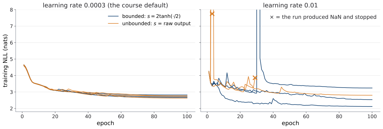
Figure 2 is the honest version of the promise. At the settings this lab trains with, the bound changes nothing you can see: of three seeds each, bounded and unbounded, none diverged and the final losses differ by less than the seed-to-seed spread. The bound is insurance, and insurance is invisible until the day it pays. At a learning rate thirty times larger, it pays: two of three unbounded runs die, none of the bounded ones do. The policy costs one line and one tanh, and you write it because the day you need it is the day you have no time to find it.
Why the head is not zero
One given decision decides whether every check below can fail at all, so it is stated. The course’s recipe card (the U0.T2 defaults, restated in §3) zero-initializes a network’s last layer wherever “output \(\approx 0\) at start” is sensible, and a coupling layer that starts as the identity is sensible. But a zero head makes \(s \equiv 0\) at initialization: the analytic log-determinant is \(0\), the automatic differentiation log-determinant is \(0\), and the two agree perfectly on nothing. The bootcamp met this twice, in U0.L3 and U0.L4. So the conditioner’s last layer starts small but nonzero, its default initialization scaled by \(0.1\): near the identity, with a log-determinant the checks can see. Measured at initialization on 64 validation points, the largest \(|\log|\det J||\) of the six-layer stack is \(0.020\); that is small, and it is not zero, and the notebook asserts the second fact before believing any agreement.
TODO 2.2 — the independent Jacobian witness
You wrote \(\log|\det J_\psi| = \sum_j s_j\). Now something that did not read your derivation computes the same number. Automatic differentiation can assemble the full \(d \times d\) Jacobian of \(z \mapsto \psi(z)\) for one example; its slogdet (the sign, and the log of the absolute value of the determinant, computed without forming the determinant itself) is what the sum must match. The recipe is two lines, and it runs in float64 on a small batch:
J = torch.func.vmap(torch.func.jacrev(single_example_map))(z)  # (B, d, d)
sign, logabsdet = torch.linalg.slogdet(J)                      # both (B,)
single_example_map sends one point (d,) to one point (d,); jacrev differentiates it; vmap batches the result. Accept under the ritual’s mixed tolerance, atol = 1e-10, rtol = 1e-8 on the largest log-determinant in the batch. Assert sign > 0 too: a coupling layer’s determinant is a product of exponentials, and a negative sign would mean the map is not the one you think.
Measured on the untrained stack, 64 points: the gap between the analytic sum and the automatic differentiation log-determinant is \(5.3 \times 10^{-16}\) against a tolerance of \(3.0 \times 10^{-10}\). On the trained stack of §3, where the largest log-determinant has grown to \(2.11\), the gap is \(5.1 \times 10^{-15}\) against \(2.1 \times 10^{-8}\). Both are float64 round-off; the sum of scales is the log-determinant.
It is tempting to call torch.autograd.functional.jacobian(f, z) on the whole batch and take one determinant. Do not. That call returns the Jacobian of the batched map \(\mathbb{R}^{Bd} \to \mathbb{R}^{Bd}\), a tensor of shape (B, d, B, d), and it is a different object from the \(B\) matrices you want. Measured, \(B = 64\): every off-diagonal block is exactly \(0\) (example \(i\) does not influence example \(j\)), so the matrix is block-diagonal and its slogdet is \(0.24336826533634\), which equals the sum of the 64 per-example log-determinants to \(4 \times 10^{-16}\). One number for the whole batch. It cannot tell you which example is wrong, its plain det is the product of \(B\) volume factors and overflows float64 for a trained flow and a large batch, and it costs \(B\) times the memory. The per-example stack is the right object, and vmap is how you get it.
TODO 2.3 — both round trips, and the cancellation
Three checks, per example, in float64: inverse(forward(z)) \(\approx\) z, forward(inverse(x)) \(\approx\) x, and logdet_fwd + logdet_inv \(\approx 0\) at matching points. Measured on the untrained stack: \(8.9 \times 10^{-16}\), \(8.9 \times
10^{-16}\) and \(2.8 \times 10^{-17}\); on the trained stack, \(9.1 \times
10^{-15}\), \(2.7 \times 10^{-15}\) and \(1.0 \times 10^{-15}\). The third check is U1.T1’s Exercise 3 executed: the inverse pass reads the same sum with the opposite sign.
3 · Stack, and train by exact maximum likelihood
Block 3, 18 minutes.
TODO 3.1 — the stack, and the sign written beside the code
A flow is a composition \(\psi = \psi_K \circ \cdots \circ \psi_1\). Its inverse undoes the layers in reverse order, and its log-determinant is the sum of the layer log-determinants, each evaluated at the point that layer sees (U1.T1 §3). Flow.forward runs the layers in order and adds; Flow.inverse runs them reversed, each through its own inverse, and adds. Masks alternate: layer \(k\) reads the half that layer \(k-1\) moved, so every coordinate moves after two layers and every coordinate can influence every other after three (U1.T1 §6).
The equality that fixes the sign is written next to the implementation, so that it is never implicit:
\[ \begin{aligned} \log p_\theta(x) &\;=\; \log p_0(z) \;+\; \log\big|\det J_{\psi^{-1}}(x)\big| , \\[2pt] z &\;=\; \psi^{-1}(x) , \end{aligned} \]
which is U1.T1’s \(\log p_0(z_0) - \sum_k \log|\det J_{\psi_k}(z_{k-1})|\) with the minus sign absorbed into logdet_inv. In code: z, logdet_inv = inverse(x), then return log_p0(z) + logdet_inv, with \(\log p_0(z) =
-\tfrac12\|z\|^2 - \tfrac{d}{2}\log 2\pi\). Checkpoint 3.1 asserts four things: that log_prob(x) equals \(\log p_0(z) - \texttt{logdet\_fwd}(z)\) at \(z = \psi^{-1}(x)\), so the sign is checked and not believed; that the witness of §2 passes on the whole six-layer stack; that both round trips pass; and that a permutation is free. U1.T1’s Exercise 1 asked you to check in your head that a coordinate swap contributes zero to the log-determinant and undoes itself. The notebook inserts a Permute layer into the stack and checks it in code: its log-determinant is exactly \(0.0\), and the stack with the swap inverts to the same \(z\).
TODO 3.2 — the closure is all you write
The loss is U1.T1’s, with the sampling subscript written out and the expectation replaced by the minibatch mean:
\[ \mathcal{L}(\theta) \;=\; -\,\mathbb{E}_{x_1 \sim q}\big[\log p_\theta(x_1)\big] \;\approx\; -\frac{1}{B}\sum_{i=1}^{B} \log p_\theta\big(x_1^{(i)}\big) . \]
Everything about the loop is the given Trainer of §0. You write the closure it needs: a module whose forward(x) returns flow.log_prob(x), and a loss module that returns minus its mean.
class LogProbModel(nn.Module):       # the Trainer calls model(x)
    def forward(self, x):
        return self.flow.log_prob(x)

class NLL(nn.Module):                # loss_fn(model(x), y); y is a placeholder
    def forward(self, logp, y):
        return -logp.mean()

opt = torch.optim.AdamW(model.parameters(), lr=3e-4, weight_decay=0.01)
sched = LambdaLR(opt, lambda s: warmup_cosine(s, total, int(0.05 * total)))
trainer = Trainer(model, opt, NLL(), "cpu", ckpt_dir="runs/...", sched=sched)
history = trainer.fit(train_loader, val_loader, epochs=500)
The settings are the course defaults (the U0.T2 recipe card, restated: AdamW at base learning rate \(3 \times 10^{-4}\), weight decay \(0.01\), linear warmup over 5% of the steps then cosine decay to \(\approx 0\), stepped per step), with \(K = 6\) layers and conditioners of width 64, for 26,508 parameters. The budget is 500 epochs of 16 steps at batch size 256, that is 8000 steps. The training set is two_moons(4096, 0) and the validation set two_moons(1024, 1); the validation loss selects best.pt, and nothing is ever selected on a test set because there is none.
The relative checkpoint, pre-validated
Checkpoint 3.2 asks two things. The validation NLL at the end must beat the first epoch’s by more than one nat, and the trained stack must still pass the witness and the round trips. The criterion is relative on purpose: an absolute threshold is a promise about the reader’s hardware and configuration that nobody validated, and the L3 pre-plan forbids one. The reference run, on CPU, gives the numbers of Table 2.
| Run | Params | Steps | Time (CPU) | Val NLL, epoch 1 | Val NLL, epoch 500 | Best |
|---|---|---|---|---|---|---|
| two-moons, scratch | 26,508 | 8000 | 69 s | 4.674 | 2.099 | 2.097 |
| gapped checkerboard, scratch | 26,508 | 8000 | 69 s | 6.927 | 3.387 | 3.386 |
| two-moons, Zuko RealNVP (§5) | 26,508 | 8000 | 74 s | 5.947 | 2.101 | — |
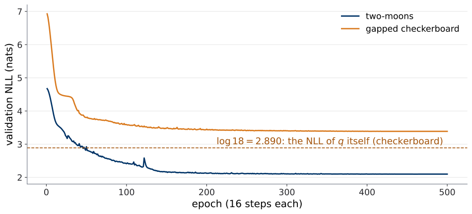
TODO 3.3 trains the same code, with the same budget, on the gapped checkerboard, and keeps the model for §4. One line changes: the generator. The checkerboard curve of Figure 3 is the first place today where a number is known that the model does not reach. For two-moons no closed-form entropy exists, so no line is drawn; for the checkerboard the optimum is exactly \(\log 18\), and the model stops \(0.50\) nats above it.
4 · Look at what you built
Block 4, 12 minutes.
Two pictures per model, both from the toy2d helpers. The density heatmap evaluates your log_prob on a \(200 \times 200\) grid, which is exact density evaluation, the thing this unit exists for. The warped grid pushes a regular grid of the source space through \(\psi^\theta\).
Two-moons
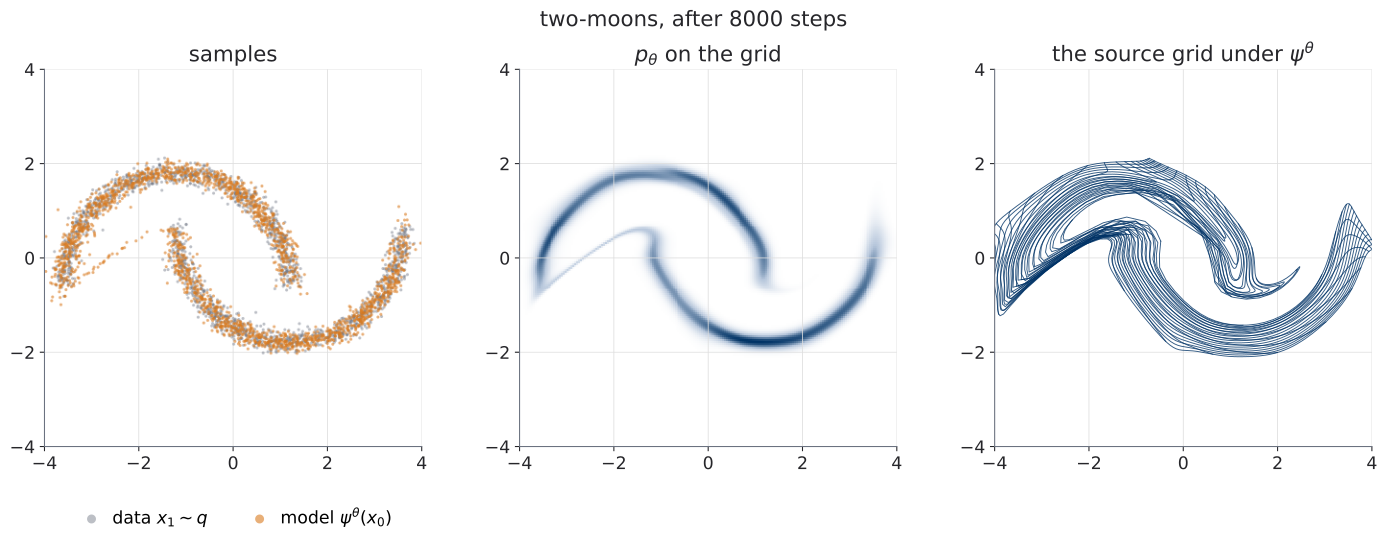
Read the right panel of Figure 4 against U1.T1’s local-volume figure. That figure pushed one small cube through a diffeomorphism and read the density change off the volume change. This panel pushes the whole source grid through the learned diffeomorphism, and the same reading holds cell by cell. The grid is one connected sheet, folded and stretched, never torn: a diffeomorphism cannot tear. Keep that sentence for the next figure.
The right panel is the end of six layers, and the two facts this block teaches are both about the composition: each layer moves one coordinate and leaves the other exactly where it was, with the roles swapping every layer; and the sheet is stretched and folded but never torn, at every stage, not only at the end. A snapshot shows the sum. The animation below shows the six summands, on the trained weights of the reference model, with the \(400\) gray source samples riding the sheet and one orange sample tracked with its running \(\log|\det J|\):
Three things in it are worth naming. The lines run off the panel and come back: after layer 1 more than half of the \(3\sigma\) source grid lies outside the window, and it returns by layer 5. The panel is a viewport, exactly as the figure’s axis limits are, and hiding what leaves it would misstate what six coupling layers do. The counter is the log-determinant of the map on screen, not a tween, and at the end of every layer it matches the per-example autodiff Jacobian of §2; in the final frame both read \(-1.105\), and they agree to \(8 \times 10^{-16}\). And the last line is the equality of §3, written in the generative direction as U1.T1 wrote it, with the numbers filled in at the tracked sample: \(\log p_\theta(x) = \log p_0(z_0) - \log|\det J_\psi(z_0)|\), that is, \(-1.737 = -2.842 - (-1.105)\).
What is drawn is the curve, not a chord through it: the figure’s \(200\) nodes per line leave \(2\)-unit chords where the trained map stretches by a factor near \(70\), so the precompute subdivides every visible segment until no drawn step exceeds \(0.12\) units, and asserts it. U1.T1’s animation of the same idea used two hand-chosen layers; this is the callback, on the model you trained.
The gapped checkerboard, and the question
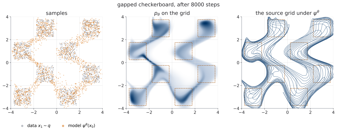
The lab asks exactly one question here, and the solution records an observation, not an explanation.
What density does the model place in the hard-zero gaps, and what happens to the grid near those regions?
Measured on the reference model, on a \(400 \times 400\) grid: \(29.8\%\) of the model’s mass lies outside the eight squares, where the data density is exactly zero; the mean density in the gaps is \(0.166\) times the mean density on the support; and along the segment joining the nearest corners of two diagonal neighbours, from \((-2.25, -2.25)\) to \((-1.75, -1.75)\), the density never drops below \(0.040\), against the uniform level \(1/18 \approx 0.056\) inside a square. The grid is stretched across every gap: the image of the source grid is one connected sheet pulled into eight bulges with material left between them. The validation NLL stops \(0.50\) nats above \(\log 18\).
Explained in U1.T2. Do not read the size of the bridge as a theorem. What is exactly impossible for this model, and what is an effect of finite capacity or of optimization, are separated in that session; today’s numbers are the observation it starts from.
The callout gives the state at the end of training, and a reader can suspect that the bridges are a transient that more training would remove. The observation the lab records is stronger than a snapshot: the mass in the gaps falls fast, then stops falling. That is a fact about a curve in time, and the animation below plays it — the reference run at sixteen checkpoints from epoch \(1\) to \(500\), the density on the figure’s own \(400 \times 400\) grid at one fixed colour scale, the validation NLL against \(\log 18\), and the mass outside the eight squares traced in an inset as it happens:
Three moments carry the curve. Through epoch \(30\) the model is one blurred blob that spreads over the board, and the mass outside barely moves: \(71\%\) at epoch \(1\), \(71\%\) at epoch \(30\). Between epochs \(30\) and \(50\) the squares appear and the mass outside drops from \(71\%\) to \(54\%\) — a checkpoint at epoch \(40\) is in the list so that the cross-fade never shows a state the model did not have. From epoch \(200\) the curve bends flat, \(33\%\) to \(30\%\) over the last \(300\) epochs, and it ends at the callout’s \(29.8\%\).
“And stay” is a measured claim, not a caption. The precompute asserts the plateau two ways: over the last \(40\%\) of training the mass moved by \(8.3\%\) of what the first \(10\%\) moved it, and between epochs \(200\) and \(300\), with the learning rate still above a third of its peak, it moved by \(3.2\%\) of its total drop. The second leg is there because the cosine schedule drives the learning rate to zero over the same tail, and a flat tail under a vanishing learning rate would prove nothing. If either assertion failed, the scene would not build. It ends on the question of TODO 4.3, verbatim, and says nothing about why.
5 · The library cross-check, and reading its source
Block 5, 14 minutes. Board 1 of the live session: U1.T1’s two-costs table, with “course \(\psi\)” and “library \(f = \psi^{-1}\)” written above it.
Reference for this section: (Rozet et al. 2022), version 1.5.0, pinned in environment.yml.
TODO 5.1 — Zuko’s RealNVP, same data, same budget, same Trainer
Zuko is the course’s reference implementation for discrete flows, and the course principle (L1 §2) is that a library is a cross-check, never a substitute for the from-scratch pass. Its flows are nn.Modules whose call returns a distribution: flow() is \(p_\theta\), with .log_prob and .sample. So the closure of §3 changes by one token, flow.log_prob(x) becomes flow().log_prob(x), and nothing else changes: the data, the seeds, the optimizer, the schedule, the Trainer. That is the point of a cross-check.
The direction needs a translation, and the translation is asserted rather than trusted.
| Map | Direction | Used by | |
|---|---|---|---|
| course | \(\psi\) | \(z \to x\) (source to data) | sample, your forward |
Zuko flow.transform() |
\(f = \psi^{-1}\) | \(x \to z\) (data to source) | log_prob |
Zuko flow.transform().inv |
\(\psi\) | \(z \to x\) | sample |
f.log_abs_det_jacobian(x, z) is \(\log|\det J_{\psi^{-1}}(x)|\), your logdet_inv, so Zuko’s log_prob is the same equality as §3: \(\log p_0(f(x)) + \log|\det J_f(x)|\). Measured on the 1024 validation points after training: the largest gap between that hand-assembled value and flow().log_prob(x) is \(9.5 \times 10^{-7}\) (float32), and f.inv(f(x)) returns \(x\) to \(3.3 \times 10^{-6}\). Never flip the course convention to match a library. Write \(f = \psi^{-1}\) and translate.
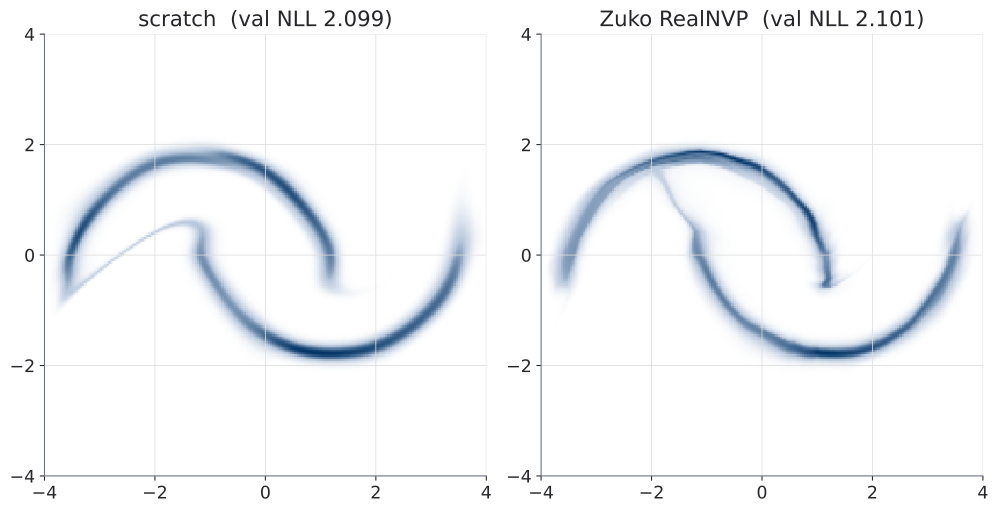
RealNVP(features=2, transforms=6, hidden_features=(64, 64)), trained by the same Trainer with the same data, seeds and schedule, validation NLL \(2.101\). The two models have the same number of parameters, 26,508, because they are the same architecture; the two densities differ in the details of the faint low-density thread and agree everywhere the data live.
The two numbers in Figure 6 are \(0.002\) nats apart. That agreement is the cross-check passing, and it says something specific: the object you wrote in §2 is the object the library ships, up to the choice of activation (SiLU here, ReLU there) and the shape of the scale bound.
TODO 5.2 — source reading: your layer in Zuko’s code
Zuko splits the layer into two classes. A lazy module, GeneralCouplingTransform, owns the mask and the conditioner (Zuko calls it the hypernetwork) and builds a transform on demand. The transform, CouplingTransform, does the arithmetic, and delegates the per-coordinate affine map to MonotonicAffineTransform. The worksheet maps your code onto theirs:
| Your code | Zuko object | What to find |
|---|---|---|
mask (True marks \(x_A\)) |
the lazy class, __init__; the transform’s split and merge |
where the mask is stored; which value marks the untouched half; how NICE alternates it across layers |
_heads |
the lazy class, meta and hyper |
what meta returns, and how the two heads are packaged |
inverse |
the transform’s _inverse; the affine map’s _inverse |
which of _call and _inverse is \(\psi\), in course notation |
logdet_fwd, logdet_inv |
log_abs_det_jacobian; call_and_ladj |
where the sum over the moved coordinates is taken; how the log-scale is bounded |
The line anchors are in the notebook, not on this page. They are generated by the notebook’s build script from the Zuko version installed in the pinned environment, and the script refuses to run against any other version. A line number written into a permanent document rots the first time the library moves; one computed at release time cannot. The four answers, in outline: the mask is a buffer, ones mark the untouched half as in your code, and NICE alternates it with torch.arange(features) % 2 == i % 2; meta is your _heads, returning \((s, t)\) packaged as a transform object; the library’s _call is \(f = \psi^{-1}\) and its _inverse is \(\psi\), with the arithmetic of your two methods and the names swapped; and the sum over the moved coordinates is taken one level up, in a DependentTransform, after the per-coordinate log-scale is expanded. The bound is a soft clip, \(\text{raw}/(1 + |\text{raw}/\log 10^{-3}|)\), which keeps \(|s| < 6.9\).
TODO 5.3 is a reserved slot: a deeper Zuko API and source exercise lands there only if U1.L2 is cut from the calendar.
6 · The same map in JAX, and the close
Block 6, 8 minutes, and skippable.
The JAX primer (U0.L5, in the self-study packet) introduced jax.jacfwd and jax.vmap. The whole generative coupling map is about fifteen lines of JAX, and the witness of §2 is two of them:
def psi(z):                         # ONE example, (2,) -> (2,)
    x = z
    for first_is_a, ws, s_cap in params:
        ia, ib = (0, 1) if first_is_a else (1, 0)
        raw = mlp(ws, x[ia:ia + 1])
        s = s_cap * jnp.tanh(raw[0] / s_cap)
        x = x.at[ib].set(x[ib] * jnp.exp(s) + raw[1])
    return x

J = jax.vmap(jax.jacfwd(psi))(z)    # (B, 2, 2)
_, logabsdet = jnp.linalg.slogdet(J)
params holds the trained torch weights, copied over. jacfwd is forward-mode, the natural mode for a map with as many outputs as inputs; vmap batches the single-example Jacobian, as torch.func.vmap did.
Measured with the trained two-moons weights on 64 points: the JAX log-determinants agree with torch’s to \(1.1 \times 10^{-13}\) and the forward maps to \(3.9 \times 10^{-15}\). It is the same function with the same weights, in a second language, and the second language’s Jacobian is a second independent witness.
Reading the board
| On the board | Status |
|---|---|
A bijection: AffineCoupling, Flow |
Built. Both round trips pass per example, before and after training (§2). |
Exact density evaluation: Flow.log_prob |
Built and used. The sign is checked (§3); the loss of §3 trained two models; the library agrees to \(0.002\) nats (§5). |
| An independent Jacobian witness | Built, twice. torch.func (§2) and JAX (§6), per example, float64. |
| The gaps of the checkerboard | Observed, not explained. \(29.8\%\) of the mass outside the support; \(0.50\) nats above \(\log 18\) (§4). U1.T2. |
For PS1.4
PS1.4(b), assigned in U1.T1, asked for \(\log p_\theta(x_1)\) of a three-layer RealNVP in \(d = 4\) as a fully explicit expression, with every conditioner read at the correct intermediate point. Your module can check your expression. Build the three layers with the masks of PS1.4 (layers 1 and 3 read \((\xi_1, \xi_2)\) and move \((\xi_3, \xi_4)\); layer 2 the reverse), run the inverse chain by hand, evaluate your expression, and compare with Flow.log_prob. The notebook’s last cell does this for the reference implementation, and the two agree to \(1.8 \times 10^{-15}\). If yours does not, the disagreement is a specific intermediate point read by the wrong conditioner, and the chain tells you which.
Where this page reappears
| From this page | Reappears in |
|---|---|
toy2d-datasets, §1 |
U1.T2 (the checkerboard as witness); U2.L1, U2.L2, U3.L1, U3.L3 (same points, other models); U6 notebooks |
coupling-layer-scratch, §2 |
PS1.4 (verification); U1.L2 (the affine algebra, inherited) |
| The per-example Jacobian witness, §2 | U2.L1 (a Jacobian trace, where the full matrix is too expensive) |
| The direction table, §5 | every library cross-check of the course |
| The gap observation, §4 | U1.T2, opening |
Next session
The next session is a theory session (U1.T2). It opens with the checkerboard of §4 and asks what a flow built from diffeomorphisms can and cannot represent exactly. Then it opens the rest of the discrete-flow zoo and answers the depth question U1.T1 left on the board.
Before then: finish TODO 4.3 in words, and use §6 to check your PS1.4(b).