U2.T2 — CNFs, FFJORD, and the Cliffhanger
Session U2.T2 · date: see calendar-map
How to read this page. This is the hinge of the first half of the course. Since U1.T2 one question has stood on the board: what does \(\log\lvert\det J\rvert\) become in continuous time? U2.T1 built the model and its gradient and left the question where it was; U2.L1 measured what a solver costs. Today the question is answered in one line, and the price of the answer is stated so precisely that the rest of the course is a search for the way out. The page has one equation that is used until the last session (the continuity equation, §2), one identity that answers the board (§3), one algorithm (§4), one family of penalties (§5), and one question (§6).
These notes are written to be read on their own. They depend on U2.T1 (the flow map, the two-tier regularity contract, the adjoint), on U1.T2 (the two-costs table and the Hutchinson estimator of its §6), on U1.T1 (the change-of-variables theorem) and on UP.T1 (pushforward). You do not need to have attended the bootcamp.
Three papers are the sources, and all three are translated into course notation silently.1 (Chen et al. 2018) states the instantaneous change of variables as its Theorem 1 (§4) and proves it in its Appendix A; (Grathwohl et al. 2019, sec. 3) turns it into a scalable algorithm with a trace estimator; (Finlay et al. 2020, secs. 3–4) adds two penalties that can make the solve easier in practice. The adjoint of (Chen et al. 2018) and (Massaroli et al. 2020) is U2.T1’s Box U2.T1-3 and is cited here, not derived again.
| From the board | Today |
|---|---|
| What does \(\log\lvert\det J\rvert\) become in continuous time? | Answered (§3): the integral of the divergence along the trajectory. |
| Hutchinson’s estimator: proof deferred (U1.T2 §6) | Paid (§4): unbiased, with its variance, and with the probe held fixed during a solve. |
| The two-costs table: the log-determinant cell is “???” | Filled, and broken (§6): version 3. |
| New: the price of the answer | A question (§6), boxed and left on the board. |
§1 — Where the unit stands
Reference for this section: U2.T1 §1–§5, restated without proof.
The left board
The left board of today’s session is U2.T1’s table, redrawn at minute zero. One cell is marked.
| Family | Density | Sampling | Trick, and its price |
|---|---|---|---|
| NICE / RealNVP | exact, triangular | direct | coupling; depth |
| Glow | exact | direct | mixing, multi-scale |
| MAF | parallel | sequential | AR, data side |
| IAF | sequential | parallel | AR, source side |
| Residual flow | direct; series log-det | iterative | contraction, traces |
| Neural ODE | inverse: ODE solve / NFE; \(\log\lvert\det J\rvert\): ??? | ODE solve / NFE | no inverse layer to design; Lipschitz field |
U2.T1 gave this session four things; any other part of it that the page uses is cited where it is used.
- The flow map. The solution map \(\psi_t\) of \(\dot x = f(t, x)\), a family that starts at \(\psi_0 = \mathrm{id}\) and deforms continuously (U2.T1 §2).
- A regularity contract in two tiers, and the inverse by a backward solve (U2.T1, The standing regularity contract, and Invertibility by well-posedness). Tier 1 (Lipschitz in \(x\)) gives well-posedness; Tier 2 (\(C^{1}\) in \(x\)) gives the differential identities.
- The adjoint sensitivity theorem, Box U2.T1-3 (U2.T1 §4): a gradient through a solve without storing the solve.
- The generalized adjoint, for a loss that also charges the trajectory (U2.T1 §4). That remark was planted for §5 of this page.
One letter changes
Until today the field was \(f_\theta\): a generic network in a generic equation. From now on the equation carries probability, and its field earns the course’s name for a velocity. We write \(u_t\), and \(u_t^{\theta}\) when it is learned. It is said once, aloud, and observed silently after that: when a field pushes densities around, we call it \(u\) — remember the symbol table. This is not new notation. L1 §4 already defines \(u_t\) and \(u_t^{\theta}\); today is the moment the course adopts them, so that U3 opens in a language already spoken. The object is the same one: the Neural ODE of U2.T1 with \(f_\theta\) renamed.
The standing hypothesis
Tier 2 makes \(\psi_t\) differentiable in \(x_0\) once. The statements of this page are pointwise equations for the density \(p_t\), and they need \(p_t\) to be differentiable in \(x\), which asks for one more derivative of the flow. One hypothesis, stated now and named in every box that uses it, buys that.
The field \(u \colon [0,1] \times \mathbb{R}^{d} \to \mathbb{R}^{d}\) is continuous, is \(C^{2}\) in \(x\) with \(\partial_x u\) (the Jacobian of \(u\) in \(x\)) and \(\partial_x^2 u\) continuous on \([0,1] \times \mathbb{R}^{d}\), and has \(\partial_x u\) bounded (so Tier 1 holds). The initial density is \(p_0 = \mathcal{N}(0, I_d)\); any positive \(C^{1}\) density would do. Under (H), \(\psi_t\) is a \(C^{2}\) diffeomorphism, and the density \(p_t\) of \(\psi_t(X_0)\) is positive and continuously differentiable in \((t, x)\).
The course models, built from tanh and softplus, satisfy (H) whenever their weights are bounded; ReLU does not (U2.T1 §3). (H) is chosen so that every statement of the page is classical; it is not the weakest hypothesis. §2 notes that the weak form of the continuity equation needs only Tier 1, and §3 shows that the integrated identity needs only Tier 2. Where a statement uses (H), its box says so.
Why this matters later
The left board is the before-and-after image of the session: the circled cell now, and the same table at the close of §6, with the cell filled and a new cost beside it. The adoption of \(u\) is why U3.T1 can open on an equation whose symbols the students already know.
§2 — The continuity equation
No source is followed line by line in this section. The two derivations are the standard ones, and the second is the version that survives into later sessions.
The question
Take a density \(p_0\) and a field \(u_t\), and move every sample by the ODE \(\mathrm{d}x = u_t(x)\,\mathrm{d}t\). The moved samples have a density at every time. That density is the object of the whole unit.
Under (H), let \(X_0 \sim p_0\) and \(X_t = \psi_t(X_0)\). The density of the moved samples is the density \(p_t\) of \(X_t\). Equivalently, for every bounded measurable \(\varphi\), \[ \mathbb{E}_{x \sim p_t}\big[\varphi(x)\big] = \mathbb{E}_{x_0 \sim p_0}\big[\varphi\big(\psi_t(x_0)\big)\big] . \tag{1}\] Since \(\psi_t\) is a \(C^{2}\) diffeomorphism, \(p_t(x) = p_0\big(\psi_t^{-1}(x)\big)\, \big\lvert \det J_{\psi_t^{-1}}(x) \big\rvert\): the change-of-variables theorem of U1.T1 §2, applied to \(\psi_t\).
That formula is a recipe, not an equation: it needs the flow map, and the flow map is a solution of an ODE. The question of this section is whether \(p_t\) satisfies an equation written with \(u_t\) alone. It does, and there are two ways to see it. The first builds the picture; the second is the proof.
Derivation 1: conservation of mass
Fix a bounded region \(V \subset \mathbb{R}^{d}\) with a piecewise smooth boundary \(\partial V\), and let \(n\) be the outward unit normal. The mass of \(V\) at time \(t\) is \(\int_V p_t(x)\,\mathrm{d}x\), the probability that \(X_t\) lands in \(V\). Samples are neither created nor destroyed, so this mass can change only because samples cross \(\partial V\).
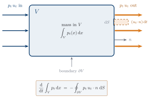
The picture gives the balance: the rate of change of the mass in \(V\) is minus the outward flux, \[ \frac{\mathrm{d}}{\mathrm{d}t} \int_V p_t(x)\,\mathrm{d}x \;=\; -\oint_{\partial V} p_t(x)\, u_t(x) \cdot n(x)\;\mathrm{d}S . \tag{2}\] Three steps finish the derivation. The left side equals \(\int_V \partial_t p_t\,\mathrm{d}x\), because \(V\) is bounded and \(\partial_t p_t\) is continuous. The divergence theorem turns the right side into \(-\int_V \nabla \cdot (p_t u_t)\,\mathrm{d}x\), because \(p_t u_t\) is \(C^{1}\) under (H); here \(\nabla\cdot g = \operatorname{tr}(\partial g/\partial x)\) is the divergence of a vector field \(g\). Together, \[ \int_V \Big[\,\partial_t p_t + \nabla \cdot (p_t u_t)\,\Big]\,\mathrm{d}x = 0 \qquad \text{for every region } V . \] The bracket is continuous, so it vanishes at every point: take \(V\) a ball, divide by its volume, and let the radius go to zero.
This derivation is the one to remember, because the control volume is the picture. It is not yet a proof: the words “mass crosses at rate density times normal velocity” are what flux means, a modelling statement. The second derivation removes that statement.
Derivation 2: the weak form
Let \(\varphi \in C_c^{\infty}(\mathbb{R}^{d})\) be a smooth test function with compact support. The proof tracks the average of \(\varphi\) over the moved samples. Its first step uses nothing but the trajectory definition.
Step 1 — the weak form. By Equation 1, the chain rule, and \(\partial_t \psi_t(x_0) = u_t(\psi_t(x_0))\), \[ \begin{aligned} \frac{\mathrm{d}}{\mathrm{d}t}\,\mathbb{E}_{x \sim p_t}\big[\varphi(x)\big] &= \mathbb{E}_{x_0 \sim p_0}\big[\nabla\varphi(\psi_t(x_0)) \cdot u_t(\psi_t(x_0))\big] \\ &= \mathbb{E}_{x \sim p_t}\big[\nabla\varphi(x) \cdot u_t(x)\big] . \end{aligned} \tag{3}\] The integrand is bounded, because \(\nabla\varphi\) has compact support and \(u\) is continuous. Equation 3 holds under Tier 1 alone, with \(\mathbb{E}_{x \sim p_t}\) read as the expectation under the law of \(X_t\). It is the form that survives when the density is not smooth, and the one a later session needs.
Step 2 — integration by parts. Write the right side of Equation 3 as an integral and move the derivative from \(\varphi\) to \(p_t u_t\): \(\int p_t\,\nabla\varphi \cdot u_t\,\mathrm{d}x = -\int \varphi\,\nabla\cdot(p_t u_t)\,\mathrm{d}x\). [C1] Which boundary term appears here, why does it vanish, and which regularity of \(p_t u_t\) is used? Stated, not proved. The clinic recording fills this step completely.
Step 3 — collect. The left side of Equation 3 equals \(\int \varphi\,\partial_t p_t\,\mathrm{d}x\), because \(\partial_t p_t\) is continuous and \(\varphi\) has compact support. Therefore \[ \int \varphi(x)\,\Big[\,\partial_t p_t(x) + \nabla\cdot\big(p_t u_t\big)(x)\,\Big]\,\mathrm{d}x = 0 \] for every test function \(\varphi\).
Step 4 — localize. [C2] Why does “zero against every test function” mean “zero at every point”? Stated, not proved: it is the fundamental lemma of the calculus of variations, and the clinic recording fills it completely.
The gaps are not exercises. They are filled, in full, in the recorded clinic (continuity-proof-clinic-recording), and that recording is required viewing before U3.T1.
The box
Theorem. Under (H), let \(p_t\) be the density of \(\psi_t(X_0)\) with \(X_0 \sim p_0\). Then \(p_t\) is positive and \(C^{1}\) on \([0,1] \times \mathbb{R}^{d}\), and for every \((t, x)\) \[ \partial_t p_t(x) + \nabla \cdot \big(p_t(x)\, u_t(x)\big) = 0 . \tag{4}\] The weak form Equation 3 holds under Tier 1 alone.
This exact equation is the foundation of everything after the break. U3 begins by reading it in the other direction.
That is the whole of what is said today about reading it in the other direction (forward tag: U3.T1).
What each derivation used. The balance needs \(\partial_t p_t\) continuous and \(p_t u_t\) of class \(C^{1}\), so that the divergence theorem applies: that is (H). The weak form Equation 3 needs only the trajectory definition: that is Tier 1. Turning the weak form into the pointwise equation Equation 4 is run under (H). The clinic draws this map once, and U3 states its theorems under the same standing hypotheses.
A worked example: a linear field on the line
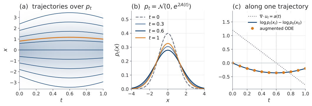
Take \(d = 1\), \(u_t(x) = a(t)\,x\) with \(a(t) = 1.2 - 2t\), and \(p_0 = \mathcal{N}(0, 1)\). The ODE \(\dot x = a(t)\,x\) has the flow map \(\psi_t(x_0) = x_0\,e^{A(t)}\) with \(A(t) = \int_0^{t} a(\tau)\,\mathrm{d}\tau = 1.2\,t - t^{2}\). A linear map sends a standard Gaussian to a Gaussian, so \(p_t = \mathcal{N}\big(0, e^{2A(t)}\big)\), and \(\tfrac{\mathrm{d}}{\mathrm{d}t}\log e^{A(t)} = a(t)\). Check Equation 4 by direct differentiation: \[ \begin{aligned} \partial_t p_t(x) &= a(t)\Big(x^{2} e^{-2A(t)} - 1\Big)\,p_t(x), \\ \nabla\cdot\big(p_t u_t\big)(x) &= \partial_x\big(a(t)\,x\,p_t(x)\big) \\ &= a(t)\Big(1 - x^{2} e^{-2A(t)}\Big)\,p_t(x), \end{aligned} \] and the two terms cancel at every \((t, x)\).
The field expands the line until \(t = 0.6\), where \(a\) changes sign, and contracts it afterwards: the scale \(e^{A(t)}\) peaks at \(1.4333\) and ends at \(e^{A(1)} = 1.2214\). This example returns in §3, where the second identity is checked on it, and in the clinic, where both are worked from scratch.
scripts/python/fig_u2_t2_cnf.py.
Why this matters later
The continuity equation is consumed by name in U3.T1 and U3.T3, and implicitly in every later session that moves a density, including the synthesis at the end of the course. The two derivations are kept on purpose: the physical one is the picture that later arguments animate, and the weak one is the version that still holds when \(p_t\) is not smooth.
§3 — Instantaneous change of variables
Reference for this section: (Chen et al. 2018, sec. 4, Thm. 1) states the identity; the computation below is the one a student should be able to redo at the board.
The computation
Fix a starting point \(x_0\) and its trajectory \(x_t = \psi_t(x_0)\). Under (H) the density \(p_t\) is positive and \(C^{1}\), so \(t \mapsto \log p_t(x_t)\) is differentiable. Three steps.
Step 1 — the chain rule, in \((t, x)\). The function \((t, x) \mapsto \log p_t(x)\) is \(C^{1}\), and the point \(x_t\) moves with velocity \(\dot x_t = u_t(x_t)\). Therefore \[ \frac{\mathrm{d}}{\mathrm{d}t}\,\log p_t(x_t) = \big(\partial_t \log p_t\big)(x_t) + \nabla\log p_t(x_t) \cdot u_t(x_t) . \tag{5}\]
Step 2 — expand the continuity equation. The product rule gives \(\nabla\cdot(p_t u_t) = p_t\,\nabla\cdot u_t + u_t \cdot \nabla p_t\). Divide Equation 4 by \(p_t > 0\): \[ \partial_t \log p_t = -\nabla\cdot u_t - u_t \cdot \nabla \log p_t . \tag{6}\]
Step 3 — add, and watch the transport terms cancel. Put Equation 6 into Equation 5, with every term on the right evaluated at \(x_t\): \[ \begin{aligned} \frac{\mathrm{d}}{\mathrm{d}t}\,\log p_t(x_t) &= \underbrace{-\nabla\cdot u_t - u_t \cdot \nabla \log p_t}_{\partial_t \log p_t\ \text{(continuity equation)}} \\ &\quad \underbrace{{}+ \nabla \log p_t \cdot u_t}_{\text{the observer rides with the sample}} \\ &= -(\nabla\cdot u_t)(x_t) . \end{aligned} \]
The cancellation is the beautiful step, and it has a meaning. The continuity equation says the density at a fixed place changes because mass is carried past it. An observer who rides along with a sample is carried with the mass, so the carrying term is exactly what the chain rule adds back. What is left is compression and expansion: the density seen by the rider falls where the field spreads the samples apart \((\nabla\cdot u > 0)\) and rises where it squeezes them together \((\nabla\cdot u < 0)\).
Theorem. Under (H), along every trajectory \(x_t = \psi_t(x_0)\), \[ \frac{\mathrm{d}}{\mathrm{d}t}\,\log p_t(x_t) = -(\nabla\cdot u_t)(x_t), \tag{7}\] and, integrating from \(0\) to \(1\) with \(x_1 = \psi_1(x_0)\), \[ \log p_1(x_1) = \log p_0(x_0) - \int_0^{1} (\nabla\cdot u_t)(x_t)\,\mathrm{d}t . \tag{8}\] Equivalently, \(\log\lvert\det J_{\psi_1}(x_0)\rvert = \int_0^{1} (\nabla\cdot u_t)(x_t)\,\mathrm{d}t\).
The last line is equivalent to the one above it by the change-of-variables theorem of U1.T1 applied to \(\psi_1\), which gives \(\log p_1(x_1) = \log p_0(x_0) - \log\lvert\det J_{\psi_1}(x_0)\rvert\).
The solve direction, and a sign that is easy to lose
To evaluate a density, the data point is the given. We hold \(x_1\) at \(t = 1\) and do not know \(x_0\); a backward solve finds it (U2.T1 §3).
Along the trajectory through the data point \(x_1\), the log-density correction is \[ \Delta(t) := \log p_t(x_t) - \log p_1(x_1) . \tag{9}\]
Then \(\Delta(1) = 0\), and by Equation 7 \(\dot\Delta(t) = -(\nabla\cdot u_t)(x_t)\). At the other end, \(\Delta(0) = \log p_0(x_0) - \log p_1(x_1)\), so \[ \log p_1(x_1) = \log p_0(x_0) - \Delta(0) . \tag{10}\] The state and the correction are one augmented ODE, solved together from \(t = 1\) down to \(t = 0\): \[ \frac{\mathrm{d}}{\mathrm{d}t}\begin{pmatrix} x \\ \Delta \end{pmatrix} = \begin{pmatrix} u_t(x) \\ -\nabla\cdot u_t(x) \end{pmatrix}, \qquad \begin{pmatrix} x \\ \Delta \end{pmatrix}(1) = \begin{pmatrix} x_1 \\ 0 \end{pmatrix} . \tag{11}\]
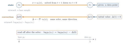
Do not start an auxiliary variable at zero and then call its terminal value “the log-likelihood”. \(\Delta(0)\) is a difference of two log-densities. The likelihood is \(\log p_0(x_0)\) minus \(\Delta(0)\). Reading \(\Delta(0)\) as the likelihood, or adding it to \(\log p_0(x_0)\), gives a wrong number, and Exercise 1 of §7 puts a size on how wrong.
For a generated sample the direction is the opposite one: start at \(x_0\), integrate forward, and Equation 8 gives, up to solver error, the model density at the generated point, at the price of the same integral.
The question on the board, answered
What does \(\log\lvert\det J\rvert\) become in continuous time?
It becomes the integral of the divergence along the trajectory: \[ \log\lvert\det J_{\psi_1}(x_0)\rvert = \int_0^{1} (\nabla\cdot u_t)(x_t)\,\mathrm{d}t . \tag{12}\] A determinant became a trace, accumulated in time. In the density it enters with a minus sign, exactly as in U1: \(\log p_1(x_1) = \log p_0(x_0) - \log\lvert\det J_{\psi_1}(x_0)\rvert\).
✔ Checked off the board.
Discrete against continuous
The same object, discrete and continuous. U1’s stack pays one determinant per block; U2’s flow pays one integral.
| U1: a stack of \(K\) blocks | U2: a flow | |
|---|---|---|
| the map | \(z_k = \psi_k(z_{k-1})\) | \(x_1 = \psi_1(x_0)\), the flow of \(u_t\) |
| the log-determinant | \(\sum_k \log\lvert\det J_{\psi_k}(z_{k-1})\rvert\) | \(\int_0^1 (\nabla\cdot u_t)(x_t)\,\mathrm{d}t\) |
| what makes it tractable | the architecture: triangular, autoregressive, a contraction | nothing is designed: the divergence is a trace (§4) |
| ancestor | the change-of-variables theorem (U1.T1) | the same theorem, in differential form |
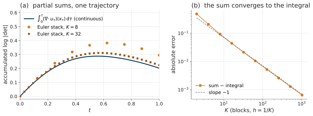
Figure 4 shows the two sides on one trajectory of the 2-D field of U2.T1’s flow-family figure: the Euler stack of \(K\) blocks, with \(h = 1/K\), against the integral. The sum converges to the integral and, from \(K = 16\) on, the error halves each time \(K\) doubles (the ratios are in the caption).
scripts/python/fig_u2_t2_cnf.py.
Why the factors of the stack become the trace of the field is PS2.2(d), below. Nothing in this table proves it; the figure only shows that it happens.
A second proof, and what it needs
The identity has a second proof that does not use the continuity equation at all.
Let \(J_t = J_{\psi_t}(x_0) = \partial\psi_t(x_0)/\partial x_0\). Under Tier 2, \(J_t\) solves the variational equation \(\dot J_t = (\partial_x u)(t, x_t)\,J_t\), \(J_0 = I\) — the equation that U2.T1’s flow-family figure integrated beside the state. Jacobi’s formula for the derivative of a determinant gives \[ \begin{aligned} \frac{\mathrm{d}}{\mathrm{d}t}\,\log\det J_t &= \operatorname{tr}\big(J_t^{-1}\dot J_t\big) \\ &= \operatorname{tr}\big((\partial_x u)(t, x_t)\big) = (\nabla\cdot u_t)(x_t), \end{aligned} \] and \(\det J_t > 0\) (U2.T1, orientation). Integrating gives Equation 12, and the change-of-variables theorem gives Equation 8.
The two routes need different things, and the difference is worth keeping. The determinant route needs only Tier 2 and gives the identity along trajectories, in its differential and its integrated form, but not the pointwise equation at a fixed \(x\). The continuity route is run under (H), and gives more: the pointwise equation for the density, and a uniqueness statement. Indeed, let \(\tilde p_t\) be any \(C^{1}\) function with \(\tilde p_0 = p_0\) that solves Equation 4. The computation of Steps 1–3, run without the logarithm so that no positivity is needed, uses the equation and nothing else, so along every trajectory \(\frac{\mathrm{d}}{\mathrm{d}t}\,\tilde p_t(x_t) = -\tilde p_t(x_t)\,(\nabla\cdot u_t)(x_t)\), which gives \(\tilde p_t(x_t) = p_0(x_0)\exp\!\bigl(-\!\int_0^{t}(\nabla\cdot u_\tau)(x_\tau)\,\mathrm{d}\tau\bigr)\). The same formula holds for \(p_t\), so \(\tilde p_t = p_t\). The density of the moved samples and the \(C^{1}\) solution of the equation with the same initial density are one object.
The example, continued
For \(u_t(x) = a(t)\,x\) the divergence is \(\nabla\cdot u_t = a(t)\) at every \(x\). So along every trajectory \(\log p_t(x_t) - \log p_0(x_0) = -A(t)\), and the correction has the same value for every data point: \(\Delta(0) = A(1) = 0.2\). Take the data point \(x_1 = 1.0\). The backward solve of Equation 11 returns \(x_0 = 0.8187\) (which is \(x_1 e^{-A(1)}\)) and \(\Delta(0) = 0.2000\). With \(\log p_0(x_0) = -1.2541\), Equation 10 gives \[ \log p_1(x_1) = -1.2541 - 0.2000 = -1.4541, \] the log-density of \(\mathcal{N}(0, e^{2A(1)})\) at \(x_1\).
Panel (c) of Figure 2 is this example: while \(a > 0\) the density seen by the rider falls, and after \(a\) changes sign it rises. The script solves Equation 11 by RK4 at five data points, and the largest error in \(\log p_1\) against the exact Gaussian is \(1.3 \times 10^{-13}\). The five values of \(\Delta(0)\) are equal, as the argument says they must be. A field whose divergence depends on \(x\) can make the data points pay different amounts.
PS2.2, assigned at the board
PS2.2 is assigned at the end of this section, once the identity has been used. It is the proof of the identity, and the bridge from U1.
Setting: \(u\) satisfies (H); \(p_0 = \mathcal{N}(0, I_d)\), smooth and positive; \(p_t\) is the density of \(\psi_t(X_0)\) and satisfies Equation 4 pointwise.
(a) Justify the total-derivative expansion of \(\mathrm{d}/\mathrm{d}t\,\log p_t(x_t)\) along a trajectory (which chain rule, applied to what function of \((t, x)\)?).
(b) Expand the continuity equation’s divergence term and carry out the cancellation in full, tracking which terms are evaluated at \(x\) versus along \(x_t\).
(c) Derive the integrated likelihood formula, including the direction-of-solve bookkeeping and all signs, for a sample given at \(t = 1\).
(d) The bridge, made rigorous: Euler-discretize the ODE and, under a small-step condition ensuring \(I + hJ\) is nonsingular and the matrix-log expansion is valid, show \(\log\lvert\det(I + hJ)\rvert = h\operatorname{tr}(J) + O(h^{2})\). Conclude in one sentence how U1’s sum of log-dets becomes U2’s divergence integral.
(e) Bonus. Where exactly did (b) use smoothness of \(p_t\), and what could fail without it? (One paragraph; no measure theory expected.)
Assigned today; released with PS2. Part (d)’s concluding sentence is the session’s thesis in your own words, and it is not in these notes.
In (d), \(J\) is the Jacobian of the field at the Euler point, \(\partial_x u(t_k, x_k)\); U1.T2 wrote it \(J_f\).
Why this matters later
The identity is applied verbatim, later in the course, to the likelihood of models whose samples come from an ODE. That one reuse is why it is proved carefully today and why PS2.2 is a problem-set slot. Part (d) is the rigorous version of the passage from residual stack to ODE, and it trains the habit of discretizing and expanding that a later problem set needs.
§4 — FFJORD: the likelihood as an augmented ODE
Reference for this section: (Grathwohl et al. 2019, sec. 3) for the algorithm and the trace estimator; (Chen et al. 2018, sec. 4) for the continuous normalizing flow it builds on.
From identity to algorithm
§3 ended on Equation 11. Replace the field \(u_t\) by a network \(u_t^{\theta}\), and that equation computes a likelihood: solve from \([x; \Delta](1) = [x_1; 0]\) backward to \(t = 0\), read off \(x_0^{\theta}(x_1)\) and \(\Delta^{\theta}_{x_1}(0)\), and combine them with Equation 10. The training loss is the average negative log-likelihood of the data, \[ \begin{aligned} \mathcal{L}_{\mathrm{NLL}}(\theta) &= \mathbb{E}_{x_1 \sim q}\Bigl[-\log p_1^{\theta}(x_1)\Bigr] \\ &= \mathbb{E}_{x_1 \sim q}\Bigl[-\log p_0\bigl(x_0^{\theta}(x_1)\bigr) + \Delta^{\theta}_{x_1}(0)\Bigr], \end{aligned} \tag{13}\] where \(q\) is the data distribution, \(p_0 = \mathcal{N}(0, I_d)\), and \(p_1^{\theta}\) is the density that the field \(u_t^{\theta}\) defines. This is a continuous normalizing flow (CNF) trained by maximum likelihood.
Training differentiates the scalar inside Equation 13 through the solve, and U2.T1 already says how. Reverse the clock with \(\tau = 1 - t\). The augmented state obeys \(\mathrm{d}y/\mathrm{d}\tau = (-u_{1-\tau}^{\theta}(x),\ +\nabla\cdot u_{1-\tau}^{\theta}(x))\), starts at the fixed value \(y(0) = [x_1; 0]\), and ends at \(y(1) = [x_0; \Delta(0)]\), where the loss is read. That is the setting of Box U2.T1-3, a terminal loss on an ODE with a fixed initial value, with a different field. Nothing new is derived. Two points deserve a sentence each. The augmented field is triangular: \(\Delta\) never feeds back into \(x\), so the \(x\)-block keeps its Tier 1 well-posedness and \(\Delta\) is a quadrature along a known trajectory. And Box U2.T1-3 asks more of \(u^{\theta}\) than (H) does. The augmented field \((-u^{\theta}, +\nabla\cdot u^{\theta})\) must satisfy Tier 1 and Tier 2 itself, so \(\nabla\cdot u^{\theta}\) must be globally Lipschitz in \(x\) and \(C^{1}\) in \((x, \theta)\). That holds if \(\partial_x^{2}u^{\theta}\) is bounded and \(\partial_\theta\partial_x u^{\theta}\) is continuous. Multilayer perceptrons with bounded weights and with activations whose first two derivatives are bounded (tanh, softplus) satisfy both; (Grathwohl et al. 2019, sec. 2.2) require the field and its first derivatives to be Lipschitz.
What the divergence costs
The divergence is the trace of the Jacobian, \(\nabla\cdot u = \operatorname{tr}(\partial_x u)\); the two notations name one object. A vector–Jacobian product (VJP) \(w^{\top}\,\partial_x u\) is one reverse-mode pass through \(u\), at about the cost of one evaluation of \(u\) (Grathwohl et al. 2019, sec. 3). Entry \((i, i)\) of the Jacobian is \(e_i^{\top}(\partial_x u)\,e_i\), so the exact trace needs one VJP per coordinate: \(d\) passes. In \(d = 2\) that is two passes, cheap enough to serve as the ground truth of the lab. For a \(32 \times 32\) colour image, \(d = 3072\), and one density evaluation would call for thousands of passes at every right-hand-side (RHS) call of the solver.
| Divergence at one RHS call | calls of \(u\) | extra passes | what it returns |
|---|---|---|---|
| exact trace | 1 | \(d\) VJPs (or \(d\) forward-mode passes) | \(\nabla\cdot u\) exactly |
| Hutchinson | 1 | 1 VJP | an unbiased estimate, with a variance |
The Hutchinson debt, paid
U1.T2 stated Hutchinson’s estimator and deferred its proof (U1.T2 §6, the boxed equation there). It is the estimator of the last row of Table 4, and today it becomes load-bearing. The box below is the same artifact, the same equation, and the same letter \(v\) for the probe, extended in place to version 2.
Let \(A \in \mathbb{R}^{d \times d}\) be any square matrix, let \(v\) be a random vector with \(\mathbb{E}_v[v v^{\top}] = I_d\) (Rademacher entries \(\pm 1\), or \(v \sim \mathcal{N}(0, I_d)\)), and write \(S = \tfrac12 (A + A^{\top})\).
(i) Unbiased. \(\mathbb{E}_{v}\big[v^{\top} A\, v\big] = \operatorname{tr}(A)\).
(ii) Only the symmetric part is seen. \(v^{\top} A\, v = v^{\top} S\, v\), and \(\operatorname{tr}(S) = \operatorname{tr}(A)\).
(iii) Variance. For Gaussian probes, \(\operatorname{Var}\big(v^{\top} A\, v\big) = 2\lVert S\rVert_F^{2}\). For Rademacher probes, \(\operatorname{Var}\big(v^{\top} A\, v\big) = 2\big(\lVert S\rVert_F^{2} - \sum_i A_{ii}^{2}\big) = 2\sum_{i \ne j} S_{ij}^{2}\). The Rademacher variance is below the Gaussian one by exactly \(2\sum_i A_{ii}^{2}\), so it is never above it.
(iv) One probe, held fixed during a solve. Let \(x_t\) be a trajectory that does not depend on \(v\), and \(A_t := (\partial_x u)(t, x_t)\), continuous on \([0,1]\). With the probe fixed on all of \([0,1]\), \[ \begin{aligned} \hat I(v) &:= \int_0^{1} v^{\top} A_t\, v\,\mathrm{d}t = v^{\top} \bar A\, v, \\ \bar A &:= \int_0^{1} A_t\,\mathrm{d}t . \end{aligned} \tag{14}\] Then \(\mathbb{E}_v\big[\hat I(v)\big] = \int_0^{1} (\nabla\cdot u_t)(x_t)\,\mathrm{d}t\), and (iii) holds with \(\bar A\) in place of \(A\).
In (iv), \(A_t\) is the Jacobian along the trajectory, the matrix that Box U2.T1-3 writes \(A(t)\). On this page \(A(t)\) is the antiderivative of the linear example, and for that field \(A_t = a(t)\).
Proof of (i). The number \(v^{\top} A v\) equals its own trace, and the trace is cyclic: \(v^{\top} A v = \operatorname{tr}(A\, v v^{\top})\). Expectation is linear and \(A\) is not random, so \(\mathbb{E}_v\operatorname{tr}(A\, v v^{\top}) = \operatorname{tr}\big(A\,\mathbb{E}_v[v v^{\top}]\big) = \operatorname{tr}(A)\). Only \(\mathbb{E}_v[v v^{\top}] = I_d\) is used; the zero mean that (Grathwohl et al. 2019, sec. 3.1) also assume is not needed. ∎
Proof of (ii). A number equals its transpose, so \(v^{\top} A v = v^{\top} A^{\top} v\); average the two. ∎
Proof of (iii). Gaussian: write \(S = Q\,\mathrm{diag}(\kappa_1, \dots, \kappa_d)\,Q^{\top}\) with eigenvalues \(\kappa_i\), and \(\tilde v = Q^{\top} v \sim \mathcal{N}(0, I_d)\). Then \(v^{\top} S v = \sum_i \kappa_i \tilde v_i^{2}\) is a sum of independent terms of variance \(2\kappa_i^{2}\) each, so its variance is \(2\sum_i \kappa_i^{2} = 2\lVert S\rVert_F^{2}\). Rademacher: since \(v_i^{2} = 1\), \(v^{\top} S v = \sum_i A_{ii} + 2\sum_{i<j} S_{ij}\, v_i v_j\), using \(S_{ii} = A_{ii}\). The products \(v_i v_j\) with \(i < j\) have mean \(0\) and variance \(1\), and they are pairwise uncorrelated, because a product of four probe entries has mean \(1\) only when the indices pair up. So the variance is \(4\sum_{i<j} S_{ij}^{2} = 2\sum_{i \ne j} S_{ij}^{2}\), and \(\lVert S\rVert_F^{2} = \sum_i A_{ii}^{2} + \sum_{i \ne j} S_{ij}^{2}\) gives the first form. ∎
Proof of (iv). The ODE of the state does not contain \(v\), so the trajectory and \(A_t\) are the same for every probe, and \(A_t\) is bounded on \([0,1]\). With \(v\) fixed, linearity of the integral gives \(\int_0^1 v^{\top} A_t v\,\mathrm{d}t = v^{\top}\big(\int_0^1 A_t\,\mathrm{d}t\big)v\). For the expectation, \(\mathbb{E}_v\int_0^1 \lvert v^{\top} A_t v\rvert\,\mathrm{d}t \le \mathbb{E}_v\lVert v\rVert^{2}\,\sup_t\lVert A_t\rVert < \infty\), so the order of \(\mathbb{E}_v\) and \(\int\) may be exchanged (Fubini), and (i) applies at every \(t\). The variance statement is (iii) applied to \(\bar A\). ∎
The probe is fixed during a solve
FFJORD’s implementation contract, which U2.L2 repeats: sample the probe once per example, for one likelihood solve; hold it fixed across every RHS call of the adaptive solver. The course adds one clause: and across every recomputation the adjoint performs. (Grathwohl et al. 2019, sec. 3.1, eq. 8) fix the probe vector for the duration of each solve to keep the dynamics deterministic within each call to the solver, and state that this adds no bias; (iv) above is that statement with its proof. There are two reasons for the contract. With \(v\) fixed, the augmented system is an ordinary deterministic ODE, so a solver sees what it expects. A probe redrawn at every call would make the right-hand side a random field, and the step-size controller would react to the randomness. And the adjoint of U2.T1 reconstructs the state backward and must see the same field it saw forward.
Two limits are part of the statement. First, (iv) is about the exact time integral. A numerical solve picks its steps from error estimates that depend on \(v\), so the computed estimate is not exactly the one that (iv) describes, and the page makes no blanket claim that every training gradient is unbiased. Second, the estimate of the log-density is unbiased for \(\log p_1(x_1)\) itself, because it is linear in \(\hat I\); it is not unbiased for \(p_1(x_1)\).
Variance, stated precisely
Part (iii) of the box is the precise form of a remark often made loosely. Rademacher probes remove the diagonal contribution to the variance, and they are no worse than Gaussian probes for every matrix, by \(2\sum_i A_{ii}^{2}\). The claim is not about “diagonal-dominant” matrices, and it is not an asymptotic statement: how much is saved depends on the share of \(\lVert S\rVert_F^{2}\) that sits on the diagonal. (Grathwohl et al. 2019, sec. 3.1.1) note that the variance grows with \(\lVert A\rVert_F^{2}\). The Gaussian formula of (iii) says what counts: the symmetric part, \(2\lVert S\rVert_F^{2} \le 2\lVert A\rVert_F^{2}\), which is zero for an antisymmetric \(A\) whatever the size of \(\lVert A\rVert_F\).
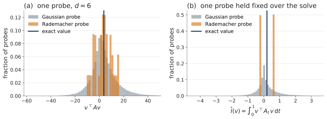
scripts/python/fig_u2_t2_cnf.py.
FFJORD, assembled
Three pieces make FFJORD, and each is now in place.
- A free-form field \(u_t^{\theta}(x)\): any network of \((t, x)\); the multilayer perceptrons described above meet the regularity that the adjoint asks for. There is no coupling pattern, no triangular Jacobian, no autoregressive order, no contraction per block.
- A stochastic divergence correction in the augmented ODE: one VJP per RHS call, with the probe fixed for the solve.
- A sensitivity method for the gradient: the adjoint of U2.T1, or direct differentiation of the solver.
What this removes is U1’s architectural bookkeeping: the design tension of the first unit is dissolved. What it keeps is that each likelihood evaluation and each training step still performs a numerical integration. §6 shows that this is not a detail but a new single cost, and states it precisely.
Why this matters later
The augmented-ODE pattern, a state with an accumulated scalar beside it, returns unchanged in U3’s likelihood computation. The v2 box is cited by U2.L2’s implementation and by any project that estimates a divergence.
§5 — Regularization: conditioning the solve
Reference for this section: (Finlay et al. 2020, secs. 3–5).
An observation protocol, and nothing more
U2.L1 logged the forward NFE of every training step of a small Neural ODE classifier: its TODO 2.3 asks for the first 100 steps of a second seed, and the reference run shows the whole run. In that reference run (seed 0, dopri5 at its defaults) the count was \(44\) on the first steps, where the field is exactly zero; it fell to \(20\) at step \(4\), reached a peak of \(134\) at step \(48\), and stood at \(122\) at step 300. That is a fact about one classifier and one solver setting. It supports one sentence, and the sentence is a protocol: a solver’s cost depends on the field, and the field can change at every optimizer step, so the number of function evaluations can change during training. It says nothing about the direction that a generative model’s cost will take. The lab measures that.
Two penalties, written as integral losses
(Finlay et al. 2020) add two integrals over the trajectory to the training loss: one charges the speed of the field, and one charges how much the field varies. With the trajectory \(x_t\) through the data point \(x_1\) and weights \(\lambda_K, \lambda_J \ge 0\), \[ \begin{aligned} \mathcal{L}_{\mathrm{reg}}(\theta) &= \mathcal{L}_{\mathrm{NLL}}(\theta) + \lambda_K\,\mathbb{E}_{x_1 \sim q}\Big[\int_0^{1} \big\lVert u_t^{\theta}(x_t)\big\rVert^{2}\,\mathrm{d}t\Big] \\ &\quad {}+ \lambda_J\,\mathbb{E}_{x_1 \sim q}\Big[\int_0^{1} \big\lVert (\partial_x u_t^{\theta})(x_t)\big\rVert_F^{2}\,\mathrm{d}t\Big]. \end{aligned} \tag{15}\] The first integral is the kinetic energy of the flow; the second uses the Frobenius norm, \(\lVert M\rVert_F^{2} = \sum_{ij} M_{ij}^{2} = \operatorname{tr}(M M^{\top})\).
The Jacobian term needs no new machinery. For a probe \(v\) with \(\mathbb{E}_v[v v^{\top}] = I_d\) and the Jacobian \(J = (\partial_x u_t^{\theta})(x_t)\), part (i) of the box applied to \(A = J J^{\top}\) gives \(\lVert J\rVert_F^{2} = \mathbb{E}_v \lVert v^{\top} J\rVert^{2}\). The row vector \(v^{\top} J\) is the VJP that the divergence estimate \((v^{\top} J)\,v\) already computes, so the penalty adds no further VJP call, and the kinetic term needs only a dot product (Finlay et al. 2020, secs. 4–5). In the estimated loss the expectation runs over \(x_1 \sim q\) and over the probe, which is fixed during each solve, exactly as in §4.
The generalized adjoint closes the loop
Both penalties are integral losses \(l(t, x, \theta) = \lambda_K \lVert u_t^{\theta}(x)\rVert^{2} + \lambda_J \lVert v^{\top} \partial_x u_t^{\theta}(x)\rVert^{2}\), and the integrand depends on \(\theta\) explicitly, through \(u_t^{\theta}\). The remark that U2.T1 planted (U2.T1 §4) is exactly this case: the adjoint equation gains the source term \(-\partial l/\partial x\), and the gradient gains the direct term \(\int_0^1 \partial l/\partial\theta\,\mathrm{d}t\). It is not enough to add only the source term to the adjoint equation: the direct term is not zero here (Exercise 3 computes both pieces for one integrand). The Jacobian penalty’s \(\partial l/\partial x\) involves second derivatives of \(u\) (that is (H)), and for \(l\) to be \(C^{1}\) in \(\theta\) it also needs \(\partial_\theta\partial_x u^{\theta}\) continuous, which smooth networks satisfy. After the substitution \(\tau = 1 - t\) of §4 nothing new is derived, and the machinery of U2.T1 certifies the training of the regularized model.
What the penalties are for, calibrated
The penalties control the speed of the field and the variation of its Jacobian along trajectories. A field that varies slowly along its trajectories is easier for a solver to follow, and in practice that can make each solve cheaper. “Cheaper” is an empirical statement and not a theorem. (Finlay et al. 2020) report, on unregularized FFJORD flows during training on CIFAR10, a clear correlation between the number of function evaluations and the Jacobian norm (their Fig. 3). No general theorem forces a lower count: the outcome depends on the model, the dataset, the solver and the tolerance. U2.L2’s optional toggle records what the course’s own runs do.
Why this matters later
This block is the course’s first statement that the shape of a flow and the cost of a solve are linked. The thread returns later in the course. The generalized-adjoint closure also certifies the machinery that the manifold seminar track uses for integral losses.
§6 — The table breaks, and the cliffhanger
Reference for this section: U2.T1 §5 for the two training routes; §4 and §5 of this page for the rest.
The table, version 3
Continuous time removes the need to design an analytic inverse or a log-determinant layer. It does not make every direction cost the same. Sampling, density and training each pay in numerical-solve work, and the per-call price differs from task to task. The left board gets its last redraw: the same table, with the circled cell filled.
| Family | Density | Sampling | Trick, and its price |
|---|---|---|---|
| NICE / RealNVP | exact, triangular | direct | coupling; depth |
| Glow | exact | direct | mixing, multi-scale |
| MAF | parallel | sequential | AR, data side |
| IAF | sequential | parallel | AR, source side |
| Residual flow | direct; series log-det | iterative | contraction, traces |
| CNF (FFJORD) | an ODE solve, plus a divergence at every RHS call | an ODE solve | free-form field; the price is the solve |
The new row hides three different accounts. The second box opens it.
| Task | what the solver integrates | per RHS call | headline count |
|---|---|---|---|
| sampling | \(x\), from \(t = 0\) to \(t = 1\) | one call of \(u_t^{\theta}\) | NFE |
| density, exact divergence | \([x; \Delta]\), from \(t = 1\) to \(t = 0\) | \(u_t^{\theta}\) and \(d\) VJPs | NFE; the VJPs are extra work |
| density, Hutchinson | \([x; \Delta]\), from \(t = 1\) to \(t = 0\), probe fixed | \(u_t^{\theta}\) and one VJP | NFE; the VJP is extra work |
| training step (MLE) | the primal likelihood solve, then a sensitivity: stored-solver backpropagation, or a second, adjoint solve | as density; the sensitivity pass takes VJPs through the augmented field, divergence term included (second derivatives of \(u_t^{\theta}\)), at every RHS call | NFE of every solve; wall-clock is the honest total |
Read the second box against the first. The currency is shared: numerical-solve work, counted in function evaluations. The price per evaluation is not. A density call evaluates the field and takes a divergence; a sampling call only evaluates the field. The two training routes are those of the 2×3 table of U2.T1 (U2.T1 §5): stored-solver backpropagation spends memory, and the adjoint spends a second solve.
The cliffhanger, stated precisely
The cost of learning is the whole difficulty, and it fits in one paragraph. This is the paragraph, verbatim. U3.T1 opens by quoting it.
MLE training of a CNF places an adaptive numerical solve inside each optimization step. Density-mode RHS calls include both \(u_t^{\theta}\) and a divergence calculation; differentiation adds either stored-solver backpropagation or a second adjoint solve. NFE is data-, parameter-, tolerance-, and solver-dependent and may drift substantially during training. The cost of learning sits inside the innermost loop.
Each clause carries one fact of this page.
- An adaptive numerical solve inside each optimization step: the loss Equation 13 is the output of a solve (§4).
- Density-mode RHS calls include both \(u_t^{\theta}\) and a divergence calculation: the two density rows of Table 6, and Table 4.
- Stored-solver backpropagation or a second adjoint solve: the two training routes of U2.T1, now priced.
- NFE is data-, parameter-, tolerance-, and solver-dependent and may drift: the observation of §5, and U2.L1’s measurement. It says “may”, and the page does not claim that it must grow.
- The innermost loop: the point of the paragraph. The expensive thing is not inside the model. It is inside the training step.
The question
Can we obtain \(u_t^{\theta}\) by regression — without ever simulating during training?
This is the last thing on the board, boxed, positioned to be photographed. The page says nothing about how it could be answered. The last sentence of the session, verbatim:
When we meet in U3.T1, you will have felt what this question is worth.
Housekeeping
PS1 is due and PS2 is released with this session (see the calendar-map). PS2.1 (U2.T1 §6) and PS2.2 (§3) are live. PS2.5 rides with the next lab, U2.L2. The asynchronous package, which holds the U2.L2 lab, the clinic recording and the shared Q&A thread, is released according to the calendar-map. The clinic recording is required viewing before U3.T1.
The board at the close
- Left board. U1.T2’s question at the top, answered and checked off in §3; the two-costs table of Table 5 beneath it. The board tells the unit’s story from top to bottom.
- Centre boards. The control-volume derivation, kept as long as possible because the picture is the session’s mnemonic; then the weak derivation with the two gap boxes [C1] and [C2]; then the cancellation of §3.
- Right board. The boxed identity Equation 7, and PS2.2 (a)–(e) as assigned. In §6, at centre right, the question of §6, boxed.
§7 — Exercises, with answers
These are for self-checking. They are not part of PS2, and no answer here contains the concluding sentence of PS2.2(d).
Exercise 1 — sign bookkeeping. Take \(d = 1\), \(u_t(x) = c\,x\) with \(c = \tfrac12\), and \(p_0 = \mathcal{N}(0, 1)\). A data point \(x_1 = 2\) is given at \(t = 1\).
(a) Solve the augmented system Equation 11 backward from \(t = 1\) to \(t = 0\) and report \(x_0\) and \(\Delta(0)\).
(b) Compute \(\log p_1(x_1)\) from Equation 10, and check it against the density of \(\mathcal{N}(0, e^{2c})\).
(c) A student starts a variable at \(0\) at \(t = 1\) with derivative \(-\nabla\cdot u_t\), adds its value at \(t = 0\) to \(\log p_0(x_0)\), and reports the sum as the log-likelihood. By how much is the report wrong?
Exercise 2 — Hutchinson on a \(2 \times 2\) matrix. Take \(A = \begin{pmatrix} 1 & 2 \\ 0 & 3 \end{pmatrix}\).
(a) Compute \(\operatorname{tr}(A)\), \(S = \tfrac12(A + A^{\top})\) and \(\lVert S\rVert_F^{2}\).
(b) Use part (iii) of Box U2.T2-3 to give the variance of \(v^{\top} A v\) for a Gaussian probe.
(c) List the four Rademacher probes, the value of \(v^{\top} A v\) for each, and the variance. Compare with (iii).
Exercise 3 — the direct term. Take \(d = 1\), \(u_t^{\theta}(x) = \theta\,x\), and the integrand \(l = \lambda\,\lVert u_t^{\theta}(x)\rVert^{2}\).
(a) Compute \(\partial l/\partial x\) and \(\partial l/\partial\theta\).
(b) Evaluate both at \(\theta = 0.8\), \(x = 1.5\), \(\lambda = 1\).
(c) Which of the two does a method miss that adds only a source term to the adjoint equation and nothing else?
Answer to Exercise 1
(a) The state solves \(\dot x = c\,x\), so \(x(t) = x_1 e^{-c(1-t)}\) and \(x_0 = x_1 e^{-c} = 1.2131\). The correction solves \(\dot\Delta = -\nabla\cdot u = -c\) with \(\Delta(1) = 0\), so \(\Delta(0) = c = 0.5\).
(b) \(\log p_0(x_0) = -\tfrac12 x_0^{2} - \tfrac12\log 2\pi = -1.6547\), and Equation 10 gives \(\log p_1(x_1) = -1.6547 - 0.5 = -2.1547\). The linear map \(x \mapsto e^{c}x\) sends \(\mathcal{N}(0,1)\) to \(\mathcal{N}(0, e^{2c})\), and \(\log\mathcal{N}(2; 0, e)\) equals the same number.
(c) The report is \(\log p_0(x_0) + \Delta(0) = -1.1547\), which is wrong by \(2\,\Delta(0) = 1.0\) nats. The error is twice the size of the correction, because the sign is flipped and not merely forgotten.
Answer to Exercise 2
(a) \(\operatorname{tr}(A) = 4\), \(S = \begin{pmatrix} 1 & 1 \\ 1 & 3 \end{pmatrix}\), and \(\lVert S\rVert_F^{2} = 1 + 1 + 1 + 9 = 12\).
(b) \(2\lVert S\rVert_F^{2} = 24\).
(c) Since \(v_1^{2} = v_2^{2} = 1\), \(v^{\top} A v = 1 + 3 + 2 v_1 v_2 = 4 \pm 2\): the probes \((1,1)\) and \((-1,-1)\) give \(6\), and \((1,-1)\) and \((-1,1)\) give \(2\). The mean is \(4 = \operatorname{tr}(A)\), and the variance is \(4\). Part (iii) gives \(2\,(12 - (1^{2} + 3^{2})) = 4\), the same number.
Answer to Exercise 3
(a) \(\partial l/\partial x = 2\lambda\theta^{2}x\) and \(\partial l/\partial\theta = 2\lambda\theta x^{2}\).
(b) \(\partial l/\partial x = 1.92\) and \(\partial l/\partial\theta = 3.60\).
(c) The second one. Adding a source term \(-\partial l/\partial x\) to the adjoint equation accounts for the first. The direct term \(\int_0^1 \partial l/\partial\theta\,\mathrm{d}t\) in the gradient is a separate contribution, and it is not zero here, because the integrand depends on \(\theta\) through \(u_t^{\theta}\).
Reading the board
| What stood on the board | State at the close |
|---|---|
| What does \(\log\lvert\det J\rvert\) become in continuous time? | Answered (§3): \(\int_0^1 (\nabla\cdot u_t)(x_t)\,\mathrm{d}t\) along the trajectory. |
| Hutchinson’s estimator, proof deferred in U1.T2 | Paid (§4), with its variance and the fixed-probe contract. |
| The two-costs table, log-determinant cell “???” | Filled, and broken (§6): version 3. |
| New: Can we obtain \(u_t^{\theta}\) by regression — without ever simulating during training? | Open. Left on the board. |
Where this page reappears
| From this page | Reappears in |
|---|---|
| The continuity equation, Box U2.T2-1, Equation 4 and Equation 3 | U3.T1 (the foundation of the unit); U3.T3 (a later use of the same equation); U7.W2 |
continuity-proof-clinic-recording (spec: the clinic of this session) |
U3.T1 (hard prerequisite) |
| Instantaneous change of variables, Box U2.T2-2 | PS2.2; U2.L2 (the likelihood bookkeeping); U3.T3 (the likelihood of an ODE-based model, by the same identity); U7.W2 |
| The log-density correction \(\Delta\), Equation 11 | U2.L2 (the variable delta_logp); U3.T3 |
| Hutchinson v2, Box U2.T2-3, and the fixed-probe contract | U2.L2 (the implementation); any project that estimates a divergence |
two-costs-table v3, Table 5 |
U3.L1 (final consumption) |
| The generalized adjoint closing the loop, §5 | U2.L2 (the optional regularization toggle); U6, manifold track |
| The cliffhanger paragraph and the boxed question, §6 | U3.T1 (quoted on the opening slide); U7.W2 |
Next session
The next session is the lab (U2.L2): a continuous normalizing flow built from scratch with the augmented system of Equation 11, with the instruments that U2.L1 installed pointed at it. It is released with the asynchronous package, beside the clinic recording. The theory session after it (U3.T1) opens from this page.
Before then: PS2.2 (§3) is assigned today, and the clinic recording is required viewing before U3.T1. For the numerics of adaptive solvers and of backward solves beyond this course, (Kidger 2022, ch. 5) remains the optional reference.
References
Footnotes
The three papers write the state as \(z\) and the field as \(f(z(t), t)\). In this course the state is \(x\) and the field that moves probability is \(u_t\) (L1 §4); \(z\) is reserved for VAE latents and is not used for the state of an ODE (the contrast table of §3 keeps U1.T1’s \(z_k\) for the states of a layer stack). The letter \(s\) stays reserved for a second clock that a later unit introduces, and the dummy variable of an integral over \([0, t]\) is \(\tau\). §1 says why the field changes its name today.↩︎