U2.T2 — CNFs, FFJORD, and the Cliffhanger

Flow-Based Generative Models · UFRJ · 2026.2

01The continuity equation

The question on the board

Since U1.T2, one question has stood on the left board:

What does \(\log\lvert\det J\rvert\) become in continuous time?

Today:

1. the equation that governs a density moved by a field;
2. the identity that answers the board;
3. the algorithm that uses it, and the estimator it needs;
4. a family of penalties that can make the solve easier;
5. the price of the answer.

Minutes 0 to 1. BOARD 1 (left, persistent): U1.T2’s question at the top, already there. Say the joint-audience sentence once: this session depends on U2.T1, U1.T2, U1.T1 and UP.T1, and on nothing from the bootcamp.

The two costs, version 2, annotated

Family	Density	Sampling	Trick, and its price
NICE / RealNVP	exact, triangular	direct	coupling; depth
Glow	exact	direct	mixing, multi-scale
MAF	parallel	sequential	AR, data side
IAF	sequential	parallel	AR, source side
Residual flow	direct; series log-det	iterative	contraction, traces
Neural ODE	inverse: ODE solve / NFE; \(\log\lvert\det J\rvert\) ???	ODE solve / NFE	no inverse layer; Lipschitz field

One cell is marked. It is today’s question.

Minutes 1 to 3. BOARD 1 as U2.T1 left it. Point at the circled cell, and say that the same table is redrawn at the end of the session with the cell filled and one more cost beside it.

One letter changes

• Until today the field was \(f_\theta\): a generic network in a generic ODE.
• From now on the ODE carries probability. Its field is \(u_t\), and \(u_t^{\theta}\) when learned.
• The object is the same: the Neural ODE of U2.T1, renamed.

When a field pushes densities around, we call it \(u\) — remember the symbol table.

Minutes 3 to 4. Say the italic sentence once, aloud, and observe the convention silently from here on. This is not new notation: L1 section 4 already defines u_t and u_t^theta. Today is the adoption moment, so that U3.T1 opens in a language already spoken.

The standing hypothesis

Today’s statements are pointwise equations for \(p_t\). They need \(p_t\) differentiable in \(x\), which asks for one more derivative of the flow than Tier 2. Here \(\partial_x u\) is the Jacobian of \(u\) in \(x\).

\(u\) is continuous on \([0,1] \times \mathbb{R}^{d}\), \(C^{2}\) in \(x\) with \(\partial_x u\), \(\partial_x^2 u\) continuous on \([0,1] \times \mathbb{R}^{d}\), and \(\partial_x u\) bounded. The initial density is \(p_0 = \mathcal{N}(0, I_d)\).

Then \(\psi_t\) is a \(C^{2}\) diffeomorphism, and the density \(p_t\) of \(\psi_t(X_0)\) is positive and \(C^{1}\) in \((t, x)\).

Every box that uses (H) says so. The weak form needs only Tier 1; the integrated identity needs only Tier 2.

Minutes 4 to 5. Why one more derivative than Tier 2: today’s statements are pointwise equations for p_t, and they need p_t differentiable in x, which asks for one more derivative of the flow. tanh and softplus models satisfy (H) whenever their weights are bounded; ReLU does not. The clinic draws the full map of which result needs which hypothesis.

The density of the moved samples

Under (H), let \(X_0 \sim p_0\) and \(X_t = \psi_t(X_0)\). The density \(p_t\) of \(X_t\) satisfies, for every bounded measurable \(\varphi\), \[ \mathbb{E}_{x \sim p_t}\big[\varphi(x)\big] = \mathbb{E}_{x_0 \sim p_0}\big[\varphi\big(\psi_t(x_0)\big)\big] . \]

Since \(\psi_t\) is a diffeomorphism, U1.T1’s change-of-variables theorem gives \(p_t(x) = p_0(\psi_t^{-1}(x))\,\lvert\det J_{\psi_t^{-1}}(x)\rvert\).

That formula needs the flow map, which is the solution of an ODE. Does \(p_t\) satisfy an equation written with \(u\) alone?

Minutes 5 to 7. The formula is a recipe and not an equation: it needs the flow map, and the flow map is the solution of an ODE. The question of the block: does p_t satisfy an equation written with u alone?

Example: a linear field on the line

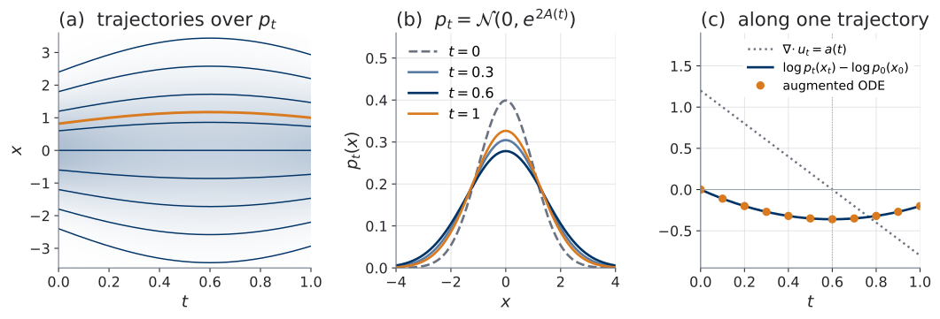
\(d = 1\), \(u_t(x) = a(t)\,x\) with \(a(t) = 1.2 - 2t\), and \(p_0 = \mathcal{N}(0,1)\). Then \[ \psi_t(x_0) = x_0\,e^{A(t)}, \qquad A(t) = 1.2\,t - t^{2}, \] so \(p_t = \mathcal{N}\big(0, e^{2A(t)}\big)\).

The field expands the line until \(t = 0.6\), then contracts it: the scale \(e^{A(t)}\) peaks at \(1.4333\) and ends at \(1.2214\).

Minutes 7 to 8. The running example of the session. Write p_t = N(0, e^{2A(t)}) on BOARD 2 under the definition. It returns twice: to check the continuity equation, and to check the second identity.

The example, pictured

Minutes 8 to 9. Panels (a) and (b) now: the trajectories x_0 e^{A(t)} over the density, and p_t at four times. The orange trajectory is the one through x_1 = 1, used in the example with numbers. Panel (c) is for the instantaneous change-of-variables block: the divergence a(t) and the change of the log-density along one trajectory; leave it until then.

Derivation 1: a control volume

Minutes 9 to 11. BOARD 2 (centre, rolling): the control-volume picture, kept as long as possible. It is the session’s mnemonic. Samples are neither created nor destroyed, so the mass in V changes only by flux through the boundary. The flux through a boundary element is density times the normal velocity, p_t u_t dot n: the samples that cross dS in time dt fill a slab of height (u_t dot n) dt.

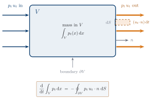
Derivation 1: the balance

\[ \frac{\mathrm{d}}{\mathrm{d}t} \int_V p_t\,\mathrm{d}x \;=\; -\oint_{\partial V} p_t\, u_t \cdot n\;\mathrm{d}S \]

1. The left side is \(\int_V \partial_t p_t\,\mathrm{d}x\).
2. The divergence theorem turns the right side into \(-\int_V \nabla\cdot(p_t u_t)\,\mathrm{d}x\), where \(\nabla\cdot g = \operatorname{tr}(\partial g/\partial x)\) for a vector field \(g\).
3. So \(\int_V [\partial_t p_t + \nabla\cdot(p_t u_t)]\,\mathrm{d}x = 0\) for every region \(V\): the bracket vanishes at every point.

This is the picture. It is not yet a proof: “flux” is a modelling statement.

Minutes 11 to 13. Every step drawn. This is the derivation the students should remember. Say the italic sentence: the second derivation is the proof.

Derivation 2: the weak form

For a smooth, compactly supported test function \(\varphi\):

\[ \begin{aligned} \frac{\mathrm{d}}{\mathrm{d}t}\,\mathbb{E}_{x \sim p_t}[\varphi(x)] &= \mathbb{E}_{x_0 \sim p_0}\big[\nabla\varphi(\psi_t(x_0)) \cdot u_t(\psi_t(x_0))\big] \\ &= \mathbb{E}_{x \sim p_t}\big[\nabla\varphi(x) \cdot u_t(x)\big] \end{aligned} \]

It uses nothing but the trajectory definition: Tier 1 is enough.

Minutes 13 to 15. Chain rule plus the derivative of psi_t equals u_t at psi_t. The integrand is bounded because grad phi has compact support. This is the version that generalizes later: it needs no smoothness of the density.

Derivation 2: two gaps

Write the right side as an integral and move the derivative onto \(p_t u_t\):

• [C1] Integrate by parts. Which boundary term? Why does it vanish? Which regularity of \(p_t u_t\) is used?
• [C2] Localize. Why does “zero against every test function” mean “zero at every point”?

Both gaps are filled, in full, in the recorded clinic. It is required viewing before U3.T1.

Minutes 15 to 17. Draw two empty boxes on BOARD 2, labelled C1 and C2, and write only the claim in each. Say it plainly: these are not exercises, they are clinic material. C1 is integration by parts with compact support; C2 is the fundamental lemma of the calculus of variations.

The continuity equation

\[ \partial_t p_t + \nabla\cdot\big(p_t\, u_t\big) = 0 \] \(p_t\) is positive and \(C^{1}\). The weak form needs only Tier 1.

This exact equation is the foundation of everything after the break. U3 begins by reading it in the other direction.

Minutes 17 to 18. PROTECTED sentence: read it verbatim and add nothing. No elaboration, no gesture at what the other direction means. Box the equation on BOARD 2 and keep it up.

Check on the example

\[ \begin{aligned} \partial_t p_t &= a(t)\Big(x^{2} e^{-2A(t)} - 1\Big)\,p_t, \\ \nabla\cdot(p_t u_t) &= a(t)\Big(1 - x^{2} e^{-2A(t)}\Big)\,p_t . \end{aligned} \] The two terms cancel at every \((t, x)\).

Minutes 18 to 20. Differentiate the log of the scale e^{A(t)}: its derivative is a. The script checks the equation by central differences on the exact density at 1,539 grid points. Overflow valve: this slide can go to the notes.

02Instantaneous change of variables

The computation, steps 1 and 2

Along a trajectory \(x_t = \psi_t(x_0)\), with \(\log p_t\) of class \(C^{1}\):

\[ \frac{\mathrm{d}}{\mathrm{d}t}\log p_t(x_t) = (\partial_t \log p_t)(x_t) + \nabla \log p_t(x_t) \cdot u_t(x_t) \]

Expand the continuity equation and divide by \(p_t > 0\):

\[ \partial_t \log p_t = -\nabla\cdot u_t - u_t \cdot \nabla \log p_t \]

Minutes 20 to 23. BOARD 2, a fresh centre panel beside the continuity equation. Step 1 is the chain rule in (t, x) for the function log p_t(x), along a point that moves with velocity u_t. Step 2 uses the product rule: div(p u) = p div u + u dot grad p. Slow down: the next slide is the beautiful step.

Step 3: the transport terms cancel

\[ \begin{aligned} \frac{\mathrm{d}}{\mathrm{d}t}\log p_t(x_t) &= \bigl(-\nabla\cdot u_t - u_t\cdot\nabla\log p_t\bigr) \\ &\quad {}+ \nabla\log p_t\cdot u_t \\ &= -(\nabla\cdot u_t)(x_t) \end{aligned} \]

Every term on the right is evaluated at \(x_t\). The first bracket is the continuity equation; the last term is the observer riding with the sample. What is left is compression and expansion.

Minutes 23 to 25. Go slowly; this is the beautiful step. The continuity equation says the density at a fixed place changes because mass is carried past it; an observer who rides with a sample is carried with the mass, so the chain rule adds the carrying term back. A rider sees the density fall where the field spreads samples apart (divergence positive) and rise where it squeezes them together.

Instantaneous change of variables

Under (H), along every trajectory \(x_t = \psi_t(x_0)\): \[ \frac{\mathrm{d}}{\mathrm{d}t}\log p_t(x_t) = -(\nabla\cdot u_t)(x_t) \] and, integrating over \([0, 1]\) with \(x_1 = \psi_1(x_0)\): \[ \log p_1(x_1) = \log p_0(x_0) - \int_0^{1} (\nabla\cdot u_t)(x_t)\,\mathrm{d}t \] Equivalently, \(\log\lvert\det J_{\psi_1}(x_0)\rvert = \int_0^{1} (\nabla\cdot u_t)(x_t)\,\mathrm{d}t\).

Cited as (Chen et al. 2018, sec. 4, Thm. 1).

Minutes 25 to 26. BOARD 3 (right, persistent from now): box the identity. PS2.2 is assigned at the end of this block, once the identity has been used. Say the sign out loud: the log-density of the data point is the base log-density MINUS the integral of the divergence.

The question that has stood on the board

What does \(\log\lvert\det J\rvert\) become in continuous time?

U1.T2 wrote it. U2.T1 circled the cell. Today it is answered.

Minutes 26 to 27. PROTECTED beat, never compressed. Pause. Point at BOARD 1, at the circled cell and at the question on top.

Answered

\[ \log\lvert\det J_{\psi_1}(x_0)\rvert = \int_0^{1} (\nabla\cdot u_t)(x_t)\,\mathrm{d}t \]

A determinant became a trace, accumulated in time. In the density it enters with a minus sign, as in U1. Checked off the board.

Minutes 27 to 29. PROTECTED beat. Physically check off the question on BOARD 1 and write the answer under it. Sign: J here is the forward Jacobian of the residual stack that U1.T2 took to the limit, so the integral enters with a plus sign (its value can have either sign); the minus sign belongs to log p_1.

Discrete against continuous

	U1: a stack of \(K\) blocks	U2: a flow
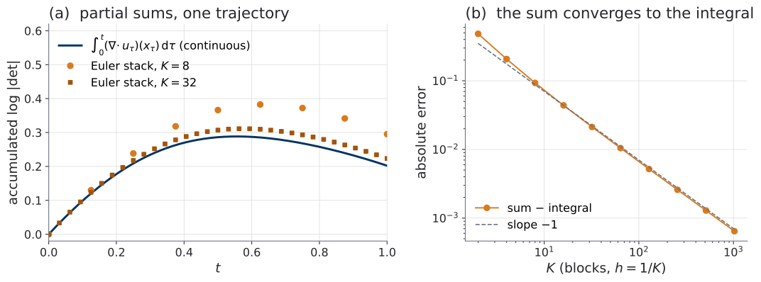
log-determinant	\(\sum_k \log\lvert\det J_{\psi_k}(z_{k-1})\rvert\)	\(\int_0^1 (\nabla\cdot u_t)(x_t)\,\mathrm{d}t\)
why tractable	the architecture	nothing is designed: a trace
ancestor	change of variables (U1.T1)	same theorem, differential form

Same object, discrete against continuous. U1 as in U1.T1: block \(k\) maps \(z_{k-1}\) to \(z_k = \psi_k(z_{k-1})\).

Minutes 29 to 30. The contrast slide. The per-block bookkeeping of U1 against one integral. Cite the change-of-variables theorem of U1.T1 as the ancestor. Why the factors become a trace is PS2.2 part (d); do not derive it here.

The sum converges to the integral

Minutes 30 to 31. Panel (a): the Euler-stack partial sums against the continuous integral on one trajectory of U2.T1’s 2-D field. Panel (b): from K = 16 on the error halves when K doubles, every halving ratio between 2.00 and 2.06. A measurement, not a proof: PS2.2 part (d) is the proof.

The solve direction

To evaluate a density, \(x_1\) is given at \(t = 1\) and a backward solve finds \(x_0\).

Along the trajectory through the data point \(x_1\): \[ \Delta(t) := \log p_t(x_t) - \log p_1(x_1) \]

Then \(\Delta(1) = 0\), \(\dot\Delta = -(\nabla\cdot u_t)(x_t)\), and \(\Delta(0) = \log p_0(x_0) - \log p_1(x_1)\):

\[ \log p_1(x_1) = \log p_0(x_0) - \Delta(0) \]

Minutes 31 to 33. To evaluate a density, the data point is the given, held at t = 1; a backward solve finds x_0. The state and the correction are one augmented ODE, solved together from t = 1 to t = 0.

One backward solve, two quantities

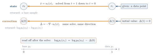
The trap: do not start a variable at \(0\) and call its terminal value “the log-likelihood”. \(\Delta(0)\) is a difference of log-densities.

Minutes 33 to 34. The state starts at the given data point and returns a base sample; the correction starts at zero and returns Delta(0). The likelihood is log p_0(x_0) MINUS Delta(0). Exercise 1 in the notes puts a size on the error of the wrong sign.

The example, with numbers

\(\nabla\cdot u_t = a(t)\) at every \(x\), so \(\Delta(0) = A(1) = 0.2\) for every data point. For \(x_1 = 1.0\):

\(x_0 = 0.8187\), \(\;\log p_0(x_0) = -1.2541\), so \[ \log p_1(x_1) = -1.2541 - 0.2000 = -1.4541 , \] the log-density of \(\mathcal{N}(0, e^{2A(1)})\) at \(x_1\).

Minutes 34 to 36. Now panel (c) of the linear-field figure: while a(t) is positive the density seen by the rider falls, and after a changes sign it rises. A field whose divergence depends on x can make the data points pay different amounts.

A second proof, and what it needs

• \(J_t = J_{\psi_t}(x_0) = \partial\psi_t(x_0)/\partial x_0\) solves \(\dot J_t = (\partial_x u)(t, x_t)\,J_t\), \(J_0 = I\) (Tier 2).
• Jacobi: \(\frac{\mathrm{d}}{\mathrm{d}t}\log\det J_t = \operatorname{tr}(J_t^{-1}\dot J_t) = (\nabla\cdot u_t)(x_t)\).
• That is the identity along trajectories, with Tier 2 only and no continuity equation.

The continuity route is run under (H), and gives more: the pointwise equation, and uniqueness.

Minutes 36 to 37. Overflow valve: this slide goes to the notes if time is short. The two routes agree. The continuity route also shows that any C1 solution of the equation with the same initial density equals p_t: the density of the moved samples and the solution of the equation are one object.

PS2.2, assigned at the board (1 of 2)

Setting: \(u\) satisfies (H); \(p_0 = \mathcal{N}(0, I_d)\), smooth and positive; \(p_t\) is the density of \(\psi_t(X_0)\) and satisfies the continuity equation pointwise.

• (a) Justify the total-derivative expansion of \(\mathrm{d}/\mathrm{d}t\,\log p_t(x_t)\) along a trajectory (which chain rule, applied to what function of \((t, x)\)?).
• (b) Expand the continuity equation’s divergence term and carry out the cancellation in full, tracking which terms are evaluated at \(x\) versus along \(x_t\).
• (c) Derive the integrated likelihood formula, including the direction-of-solve bookkeeping and all signs, for a sample given at \(t = 1\).

Minutes 37 to 39. Assign at the board now, at the end of the block: the identity has stood boxed since minute 25. BOARD 3: list (a) to (e) beside the box. The parts are the pinned wording of the course plan; the setting names (H), as in the notes.

PS2.2, assigned at the board (2 of 2)

• (d) The bridge, made rigorous: Euler-discretize the ODE and, under a small-step condition ensuring \(I + hJ\) is nonsingular and the matrix-log expansion is valid, show \(\log\lvert\det(I + hJ)\rvert = h\operatorname{tr}(J) + O(h^{2})\). Conclude in one sentence how U1’s sum of log-dets becomes U2’s divergence integral.
• (e) Bonus. Where exactly did (b) use smoothness of \(p_t\), and what could fail without it? (One paragraph; no measure theory expected.)

In (d), \(J\) is the field’s Jacobian at the Euler point, \(\partial_x u(t_k, x_k)\).

Minutes 39 to 40. Part (d)’s concluding sentence is the session’s thesis in the students’ own words. It is not in the notes, and the key states the expansion but not the sentence.

03FFJORD: the likelihood as an augmented ODE

From identity to algorithm

Replace the field \(u_t\) by a network \(u_t^{\theta}\), and solve from \([x; \Delta](1) = [x_1; 0]\) down to \(t = 0\):

\[ \frac{\mathrm{d}}{\mathrm{d}t}\begin{pmatrix} x \\ \Delta \end{pmatrix} = \begin{pmatrix} u_t^{\theta}(x) \\ -\nabla\cdot u_t^{\theta}(x) \end{pmatrix} \]

\[ \mathcal{L}_{\mathrm{NLL}}(\theta) = \mathbb{E}_{x_1 \sim q}\Bigl[-\log p_0\bigl(x_0^{\theta}(x_1)\bigr) + \Delta^{\theta}_{x_1}(0)\Bigr] \]

This is a continuous normalizing flow (CNF), trained by maximum likelihood.

Minutes 40 to 43. BOARD 2, a fresh centre panel: the augmented system, and the loss as the output of a solve. This is a continuous normalizing flow (CNF) trained by maximum likelihood. The scalar inside the expectation is the sign-safe reading of the instantaneous change-of-variables block, with the minus sign carried into the loss.

Training through the solve

• Reverse the clock, \(\tau = 1 - t\): the state \(y = [x; \Delta]\) starts at the fixed value \([x_1; 0]\) and ends at \([x_0; \Delta(0)]\), where the loss is read.
• That is the setting of Box U2.T1-3: a terminal loss on an ODE with a fixed initial value. Nothing new is derived.
• The augmented field is triangular: \(\Delta\) never feeds back into \(x\). Box U2.T1-3 asks more of \(u^{\theta}\) than (H): \(\nabla\cdot u^{\theta}\) globally Lipschitz in \(x\) and \(C^{1}\) in \((x, \theta)\). FFJORD requires the field and its first derivatives to be Lipschitz (Grathwohl et al. 2019, sec. 2.2).

Minutes 43 to 45. Cite the adjoint of U2.T1; do not re-derive it. Two honest points: the x-block keeps its Tier 1 well-posedness and Delta is a quadrature along a known trajectory; and the extra requirement (bounded second derivative in x, continuous mixed derivative in theta) holds for multilayer perceptrons with tanh or softplus activations and bounded weights.

What the divergence costs

A vector–Jacobian product (VJP) \(w^{\top}\partial_x u\) is one reverse-mode pass through \(u\), at about the cost of one evaluation of \(u\).

Divergence per RHS call	calls of \(u\)	extra passes	returns
exact trace	1	\(d\) VJPs	\(\nabla\cdot u\) exactly
Hutchinson	1	1 VJP	unbiased, with variance

NFE counts calls of \(u\). The VJPs are extra work, visible in wall-clock time, and are not extra NFE.

Minutes 45 to 48. The exact trace needs one VJP per coordinate, since entry (i, i) of the Jacobian is e_i transpose times the Jacobian times e_i. In d = 2 that is two passes: the ground truth of the lab. For a 32 by 32 colour image d = 3072. Overflow valve: the exact-trace cost accounting moves to the notes.

The Hutchinson debt, paid

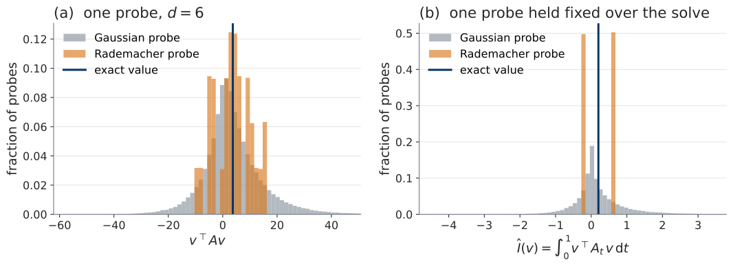
\(A \in \mathbb{R}^{d \times d}\), \(\mathbb{E}_v[v v^{\top}] = I_d\) (Rademacher or Gaussian), \(S = \tfrac12(A + A^{\top})\).

(i) Unbiased: \(\mathbb{E}_v[v^{\top} A\, v] = \operatorname{tr}(A)\).

(ii) Symmetric part only: \(v^{\top} A\, v = v^{\top} S\, v\).

(iii) Variance. Gaussian: \(2\lVert S\rVert_F^{2}\). Rademacher: \(2\big(\lVert S\rVert_F^{2} - \sum_i A_{ii}^{2}\big)\).

The Rademacher variance is below the Gaussian one by exactly \(2\sum_i A_{ii}^{2}\), so it is never above it. Version 1 is U1.T2’s box, “Hutchinson’s trace estimator”; its proof was deferred to today.

Minutes 48 to 51. The box of U1.T2, same equation, same letter v, extended in place to v2: cite the U1.T2 box on the slide. Proof of (i) in two lines on BOARD 2: the number v-transpose A v equals its own trace; the trace is cyclic, so it equals tr(A v v-transpose); expectation is linear. Only E[v v transpose] = I is used.

One probe, held fixed during a solve

Let \(x_t\) not depend on \(v\), and \(A_t = (\partial_x u)(t, x_t)\). With one probe fixed on \([0,1]\): \[ \hat I(v) = \int_0^{1} v^{\top} A_t\, v\,\mathrm{d}t = v^{\top}\bar A\,v, \qquad \bar A = \int_0^{1} A_t\,\mathrm{d}t . \] \(\mathbb{E}_v[\hat I(v)] = \int_0^{1}(\nabla\cdot u_t)(x_t)\,\mathrm{d}t\), and (iii) holds with \(\bar A\).

Fubini: \(\mathbb{E}_v\lVert v\rVert^{2} = d < \infty\) and \(\sup_t\lVert A_t\rVert < \infty\). Here \(A_t\) is the Jacobian along the trajectory (Box U2.T1-3 writes it \(A(t)\)); on this page \(A(t)\) is the antiderivative of the linear example, and for that field \(A_t = a(t)\).

Minutes 51 to 53. The interchange assumptions are on the slide on purpose: with integrability and Fubini, the time-integrated trace correction stays unbiased in expectation over the probe. Do not promote this to a blanket claim that every training gradient is unbiased.

Short proofs

• (i) \(v^{\top} A v = \operatorname{tr}(A\, v v^{\top})\), so \(\mathbb{E}_v\,v^{\top} A v = \operatorname{tr}\big(A\,\mathbb{E}_v[v v^{\top}]\big) = \operatorname{tr}(A)\).
• (ii) A number equals its transpose: \(v^{\top} A v = v^{\top} A^{\top} v\). Average the two.
• (iii) Gaussian: \(v^{\top} S v = \sum_i \kappa_i \tilde v_i^{2}\) (\(S = Q\,\mathrm{diag}(\kappa)\,Q^{\top}\), \(\tilde v = Q^{\top} v\)), variance \(2\sum_i \kappa_i^{2}\). Rademacher: \(v_i^{2} = 1\) leaves \(2\sum_{i<j} S_{ij} v_i v_j\), with pairwise uncorrelated products.

The proof of (i) needs no zero mean: only \(\mathbb{E}_v[v v^{\top}] = I_d\).

Minutes 53 to 54. Overflow valve: this slide, and the Fubini line of the previous one, go to the notes. FFJORD assumes zero mean and identity covariance; the proof uses only the second moment.

The contract for the probe

Contract. One probe per example, for one likelihood solve, held fixed across every RHS call of the adaptive solver (Grathwohl et al. 2019, sec. 3.1, eq. 8). The course adds: and across every recomputation of the adjoint.

• A deterministic augmented ODE is what a solver expects. A probe redrawn per call is a random field.
• The adjoint reconstructs the state backward and must see the field it saw forward.

Limits. The statement is about the exact integral: a solver’s steps depend on \(v\). No blanket claim that every training gradient is unbiased. The estimate is unbiased for \(\log p_1\), not for \(p_1\).

Minutes 54 to 57. The paper keeps one probe vector for the duration of each solve to keep the dynamics deterministic within each call to the solver. Cite the paper’s section and equation 8, and do not quote the authors’ code comment: it is not in the paper.

Variance, measured

Minutes 57 to 59. Panel (a): a fixed 6 by 6 matrix; closed forms 125.5 (Gaussian) and 43.50 (Rademacher); measured 125.4 and 43.52, each within four standard errors, and the Rademacher closed form reproduced by exact enumeration of all 64 probes. The claim is “never above”, for every matrix; it is not about diagonal-dominant matrices. Panel (b): the fixed-probe integral on U2.T1’s 2-D field.

FFJORD, assembled

• A free-form field \(u_t^{\theta}\): no coupling pattern, no triangular Jacobian, no contraction.
• A stochastic divergence correction: one VJP per RHS call, probe fixed for the solve.
• A sensitivity method: the adjoint of U2.T1, or direct differentiation of the solver.

The design tension of U1 is dissolved. Each likelihood and each training step still performs a numerical integration.

Minutes 59 to 60. Say the last sentence and hold it: it is the setup for the last block, where a new single cost takes the place of the old design tension.

04Regularization: conditioning the solve

An observation protocol

U2.L1, TODO 2.3 and its reference run: the forward NFE of a small Neural ODE classifier, at every training step (seed 0, dopri5 at its defaults).

first steps	at step 4	peak	at step 300
44	20	134 (step 48)	122

A solver’s cost depends on the field, and the field can change at every optimizer step. The count can change during training. No direction is claimed.

Minutes 60 to 63. Recall U2.L1 only as an observation protocol. It is a fact about one classifier and one solver setting. Do not presuppose the direction a generative model’s cost will take: the lab measures it.

Two penalties

(Finlay et al. 2020): charge the trajectory \(x_t\) through \(x_1\), for the speed and the variation of the field, with weights \(\lambda_K, \lambda_J \ge 0\).

\[ \begin{aligned} \mathcal{L}_{\mathrm{reg}}(\theta) &= \mathcal{L}_{\mathrm{NLL}}(\theta) + \lambda_K\,\mathbb{E}_{x_1 \sim q}\Big[\int_0^{1} \lVert u_t^{\theta}(x_t)\rVert^{2}\,\mathrm{d}t\Big] \\ &\quad {}+ \lambda_J\,\mathbb{E}_{x_1 \sim q}\Big[\int_0^{1} \lVert (\partial_x u_t^{\theta})(x_t)\rVert_F^{2}\,\mathrm{d}t\Big] \end{aligned} \]

For \(J = (\partial_x u_t^{\theta})(x_t)\): \(\lVert J\rVert_F^{2} = \mathbb{E}_v\lVert v^{\top}J\rVert^{2}\), and \(v^{\top}J\) is the VJP the divergence estimate already computes: no extra VJP call (Finlay et al. 2020, secs. 4–5).

Minutes 63 to 66. Kinetic energy and the Frobenius norm of the Jacobian, both integrals over the trajectory. The identity for the Frobenius norm is part (i) of the Hutchinson box applied to A = J J-transpose. The kinetic term needs one dot product.

The generalized adjoint closes the loop

• Both penalties are integral losses \(l(t, x, \theta)\), and the integrand depends on \(\theta\) explicitly, through \(u_t^{\theta}\).
• U2.T1’s remark covers exactly this: the adjoint equation gains \(-\partial l/\partial x\), and the gradient gains \(\int_0^1 \partial l/\partial\theta\,\mathrm{d}t\).
• It is not enough to add only a source term to the adjoint equation.

Nothing new is derived: the machinery planted in U2.T1 certifies the training of the regularized model.

Minutes 66 to 69. The generalized-adjoint payoff must include BOTH terms: the state-gradient source term and the explicit parameter derivative of the integrand. Do not summarize it as merely adding one term to the adjoint ODE. Exercise 3 in the notes computes both pieces for one integrand. Overflow valve for this block: compress to 6 minutes by keeping the two-penalties slide and this one, dropping the observation-protocol and calibration slides, and saying the seed sentence aloud.

What the penalties are for

• They control the speed of the field and the variation of its Jacobian along trajectories.
• A field that varies slowly is easier for a solver to follow, and in practice that can make a solve cheaper.
• “Cheaper” is an empirical result, not a theorem: (Finlay et al. 2020) report, on unregularized FFJORD flows during training on CIFAR10, a clear correlation between NFE and the Jacobian norm.

Hold on to straightness/easy-to-integrate dynamics as a virtue — it returns later.

Minutes 69 to 72. The seed, planted in one sentence and hard-stopped: do not name anything it returns as, and do not elaborate. U2.L2’s optional toggle records what the course’s own runs do; whether the NFE falls is measured there, not asserted here.

05The table breaks

The two costs, version 3

Family	Density	Sampling	Trick, and its price
NICE / RealNVP	exact, triangular	direct	coupling; depth
Glow	exact	direct	mixing, multi-scale
MAF	parallel	sequential	AR, data side
IAF	sequential	parallel	AR, source side
Residual flow	direct; series log-det	iterative	contraction, traces
CNF (FFJORD)	ODE solve + divergence per call	ODE solve	free-form field; the price is the solve

Minutes 72 to 76. BOARD 1: draw the filled row beneath the circled cell, then cross out the circle. Continuous time removes the need to design an inverse or a log-determinant layer; it does not make every direction cost the same.

Where the numerical work sits

Task	integrates	per RHS call	headline
sampling	\(x\), \(0 \to 1\)	\(u_t^{\theta}\)	NFE
density, exact	\([x; \Delta]\), \(1 \to 0\)	\(u_t^{\theta}\) and \(d\) VJPs	NFE; VJPs extra
density, Hutchinson	\([x; \Delta]\), \(1 \to 0\)	\(u_t^{\theta}\) and 1 VJP	NFE; VJP extra
training step	solve; backprop or adjoint	as density, then differentiated	NFE, all solves

NFE is the headline count; wall-clock is the honest total.

Minutes 76 to 80. The repair of the old claim: sampling and density do NOT cost the same per evaluation. A density call evaluates the field and takes a divergence; a sampling call only evaluates the field. The two training routes are the 2 by 3 table of U2.T1: stored-solver backpropagation spends memory, the adjoint spends a second solve.

The cliffhanger

MLE training of a CNF places an adaptive numerical solve inside each optimization step. Density-mode RHS calls include both \(u_t^{\theta}\) and a divergence calculation; differentiation adds either stored-solver backpropagation or a second adjoint solve. NFE is data-, parameter-, tolerance-, and solver-dependent and may drift substantially during training. The cost of learning sits inside the innermost loop.

Minutes 80 to 84. PROTECTED beat, never compressed. Read it verbatim, slowly. U3.T1 opens by quoting this paragraph. Then walk the clauses once: the solve in the loss; the divergence per call; the two training routes; “may drift”, which is not “must grow”; the innermost loop, which is the point.

The question

Can we obtain \(u_t^{\theta}\) by regression —
without ever simulating during training?

Minutes 84 to 87. PROTECTED beat. Write the question on BOARD 3 at centre right, boxed, positioned to be photographed. It is the last thing on the board before the asynchronous week. Say nothing about how it could be answered. Not even a gesture.

Housekeeping, and the last sentence

• PS1 is due and PS2 is released with this session (see the calendar-map). PS2.1 and PS2.2 are live; PS2.5 rides with the next lab, U2.L2.
• The asynchronous package (the U2.L2 lab, the clinic recording, the Q&A thread) is released per the calendar-map.
• The clinic recording is required viewing before U3.T1.

When we meet in U3.T1, you will have felt what this question is worth.

Minutes 87 to 90. Housekeeping in three minutes, then the closing line verbatim, and out. The problem-set and release logistics live in the calendar-map; do not repeat dates here.

References

Chen, Ricky T. Q., Yulia Rubanova, Jesse Bettencourt, and David Duvenaud. 2018. “Neural Ordinary Differential Equations.” In Advances in Neural Information Processing Systems. https://arxiv.org/abs/1806.07366.

Finlay, Chris, Jörn-Henrik Jacobsen, Levon Nurbekyan, and Adam M. Oberman. 2020. “How to Train Your Neural ODE: The World of Jacobian and Kinetic Regularization.” In International Conference on Machine Learning. https://arxiv.org/abs/2002.02798.

Grathwohl, Will, Ricky T. Q. Chen, Jesse Bettencourt, Ilya Sutskever, and David Duvenaud. 2019. “FFJORD: Free-Form Continuous Dynamics for Scalable Reversible Generative Models.” In International Conference on Learning Representations. https://arxiv.org/abs/1810.01367.