U2.L1 — Solvers and Adjoints in Practice

Flow-Based Generative Models · UFRJ · 2026.2

01Orientation and the entry quiz

Where this session sits

Session	Role
U2.T1	the adjoint theorem, and a table of two gradient strategies whose cells were arguments
U2.L1 — today	every cell of that table measured, on a classifier where nothing hurts
U2.L2	the same instruments, pointed at a generative model

You learn the instruments on a problem where nothing is at stake, so that the next reading means something.

Zero to ten minutes for the orientation block. Board: an empty list titled “instrument panel” on the right; it fills one line per block. U2.T1’s open question stays in its corner, untouched: do not read it, do not erase it. Notebook on the projector from here on; the deck is the map.

Six instruments you leave with

1. An NFE counter: three lines.
2. NFE-against-quality axes, on two metrics that disagree.
3. NFE drift across training.
4. A peak-memory protocol for one forward-and-backward pass.
5. A gradient-fidelity table: two routes against one witness.
6. Honest timing: compile apart from steady state.

Nothing today is about generative models. The instruments come first.

Read the six once. Each block adds one line to the board’s panel; by the debrief the list is complete and the closing sentence points it at U2.L2.

Given code, and a loop written out

Module	Built in	Used today
common/toy2d.py	U1.L1, frozen	two_moons(n, seed)
common/odesolve.py	U0.L5, frozen	odeint, with .nfe
common/train.py	U0.L1, U0.L2	set_seed only

The labels come from the frozen contract (first n // 2 rows = upper moon):

x = two_moons(n, seed)
y = (torch.arange(n) >= n // 2).long()

The training loop is written out: the NFE counter must be read between the forward solve and the backward pass of every step.

Joint sessions use bootcamp code as given code with its contract written out; attendance is never required. The frozen generator does not change; its docstring already fixes the row order. The reference script, scripts/python/fig_u2_l1_instruments.py, checks it: mean second coordinate 0.85 on label 0, −0.97 on label 1.

Where the numbers go

MLflow, deployed locally: sqlite:///mlflow.db beside the notebook.

• Experiment U2; one run per block.
• Tags session=U2.L1 and block=<n>; the resolved configuration as parameters.
• Curves logged after the loop, in one batch. The loop times every step (median 53 ms); a SQLite write inside it would be part of what it times.

Same departure as U1.L1; here the reason is that the loop times itself. The run stands alone either way.

The entry quiz: six questions

1. What does NFE count, and why is it reported for every solve?
2. Where does rtol dominate, and where atol?
3. Why is a step rejected, and what does a rejection cost?
4. What is dopri5?
5. What decides the cost of a fixed-step solve? Of an adaptive one?
6. What does stiff mean, loosely?

Four or more right: go on. Fewer: read U0.T5, Adaptive stepping and Stability, before the sweep block.

Five minutes, on paper, self-graded; answers on the last page of the notebook and at the end of the notes. The classifier block does not need the quiz; the sweep block does. For self-study students this is where the packet pays.

02A Neural ODE classifier on two moons

The model

\[ \begin{aligned} \dot x(t) &= f_\theta\big(t, x(t)\big),\quad x(0) = x_0,\quad t \in [0,1],\\ \text{logits} &= W\,\psi_1(x_0) + b \end{aligned} \]

• \(f_\theta(t, x)\): an MLP on \([x; t]\), two hidden layers of 32, \(\tanh\). With the head, 1,256 parameters.
• The state stays in the plane, \(\mathbb{R}^2\): a picture of the trajectories is a picture of the state, not a projection.
• The activation is smooth (\(\tanh\)): \(f_\theta\) is \(C^1\) in \((t, x, \theta)\) and globally Lipschitz in \(x\), uniformly in \(t\): both tiers of U2.T1’s contract. Tier 2 is what the adjoint assumes.

Ten to thirty minutes for the classifier block. Here x_0 is an input point: a classifier’s flow has no generative direction, so the course’s time arrow (noise at t = 0, data at t = 1) does not apply. This is U2.T1’s Neural ODE used as a feature map. Why not an 8-dimensional state: a projection of 8-D curves onto a plane can show crossings that do not exist, and today’s checkpoint makes a claim about the state.

The loss, and what the flow must do

\[ \ell(\theta) = \mathbb{E}_{(x_0, y) \sim \mathcal{D}_{\mathrm{train}}} \Big[ -\log \operatorname{softmax}\big(W\,\psi_1(x_0) + b\big)_{y} \Big] \]

\(\mathcal{D}_{\mathrm{train}}\): the empirical (uniform) distribution of the 512 labelled training points. Each term is U2.T1’s terminal loss \(L_y\big(x(1)\big)\), with \(L_y\) = head + cross-entropy against \(y\).

The head alone, on the raw inputs: 89.4% test accuracy. No line separates the moons; the rest is the flow’s work.

The head’s parameters enter only through L_y, so their gradient needs no backward solve. The fidelity check later draws its direction over the field’s parameters only (v is zero on the head’s parameters): all three routes computed on the N-step grid pass through the head from the same endpoint, so the head’s term would be the same in each of them and would only dilute the gaps.

TODO 1.1 — the NFE counter

class NFECounter(nn.Module):
    def __init__(self, f):
        super().__init__()
        self.f = f
        self.nfe = 0                 # 1
    def forward(self, t, x):
        self.nfe += 1                # 2
        return self.f(t, x)          # 3

A module holding the field, so its parameters are the field’s. It counts every call: stages, start-up calls, and the adjoint’s backward calls. Checkpoint 1.1: Euler with \(N\) steps must report \(N\); torchdiffeq’s rk4 must report \(4N\).

Board, panel line 1: NFE counter. Reset to zero before a solve, read after. The checkpoint is arithmetic the solver cannot fake.

TODO 1.2 — train, and read the gauges

for step in range(300):
    model.field.nfe = 0
    logits = model(x, method="dopri5")
    nfe_fwd = model.field.nfe
    loss = F.cross_entropy(logits, y)
    opt.zero_grad(set_to_none=True)
    loss.backward()
    opt.step(); sched.step()
    nfe_bwd = model.field.nfe - nfe_fwd

dopri5 at its defaults: rtol \(= 10^{-7}\), atol \(= 10^{-9}\). Full batch, 512 points. Record the loss, the accuracy, the forward NFE, the backward NFE and the seconds of every step.

Direct backprop through the adaptive solver. The backward NFE is the surprise to plant: it will read zero.

Settings, and one deviation in writing

The U0.T2 recipe card: AdamW, weight decay 0.01, 3% warmup, cosine decay, per step. Base rate: \(3 \times 10^{-3}\), not the card’s \(3 \times 10^{-4}\).

Base rate	Steps	CPU time	Loss	Accuracy
\(3 \times 10^{-4}\) (card)	1500	77 s	0.0275	99.6%
\(3 \times 10^{-3}\)	300	15.1 s	0.0032	100.0%

Loss and accuracy on the training set; CPU time on one thread. At step 300 of the card-rate run the loss is still 0.287. The card rate, with five times the steps, ends 8.5 times higher. Test accuracy of the \(3 \times 10^{-3}\) run: 100.0%.

Test NFE at the defaults: 116. Backward NFE: zero, at every step.

A lab block has twenty minutes; the card allows a deviation in writing with a reason, and the reason is the table. Direct backprop replays the recorded operations; it never evaluates the field again. Keep that zero for the memory and fidelity block.

Why the head starts at zero

Card item 3: zero the last layer where “output \(\approx 0\) at start” is sensible. Two last layers qualify.

• The field’s: the flow starts at the identity.
• The head’s: the first prediction is uniform, loss \(\log 2\).

Measured: with PyTorch’s default head, seeds 2 and 3 of five stalled at every rate tried (final training loss 0.23 or above; every other run 0.048 or below). With the head at zero, 10 seeds of 10 reached 100%.

Rates tried: 3e-3 for 300 steps, 1e-3 for 600, 3e-4 for 1500. Explanation, not theorem: a random head fixes a direction before the flow learns anything, and a flow of the plane cannot move points through each other to repair it. The cost: at initialization every field gradient is exactly zero, so a gradient check there would measure nothing; the fidelity checks use the trained model.

Checkpoint 1 — the state, in the plane

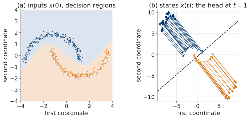
Left: every fifth test input; regions from one solve per grid point. Right: hollow \(t = 0\), filled \(t = 1\), dashed the head’s line.

Left: decision regions in input space. Right: forty trajectories in the actual state space, and the head’s line at t = 1. The flow moves the classes apart until a line separates them. Hollow markers at t = 0, filled at t = 1.

Uniqueness, as a check

Under U2.T1’s Tier 1 (Picard–Lindelöf), two distinct trajectories never occupy the same state at the same time. Read over all 2,096,128 test pairs and 41 times:

\[ 0.41 \;\le\; \frac{\lvert x^{(i)}(t) - x^{(j)}(t)\rvert}{\lvert x^{(i)}(0) - x^{(j)}(0)\rvert} \;\le\; 21.4 . \]

Paths drawn in the plane may still cross: the field depends on \(t\), and a crossing of paths happens at different times. None of the 40 drawn paths do; yours may, and that is not a contradiction.

A reading with a stated floor, not a new theorem: the script asserts a floor of 0.1, and the measured floor is 0.41. The count of drawn crossings is recorded by the script: zero.

Optional — your RK4 against the library’s

\(N\)	odesolve RK4	torchdiffeq rk4	the two RK4s
8	\(5.4 \times 10^{-3}\)	\(5.0 \times 10^{-3}\)	\(3.4 \times 10^{-4}\)
16	\(4.3 \times 10^{-4}\)	\(4.1 \times 10^{-4}\)	\(2.5 \times 10^{-5}\)
32	\(3.1 \times 10^{-5}\)	\(2.9 \times 10^{-5}\)	\(1.6 \times 10^{-6}\)
64	\(2.1 \times 10^{-6}\)	\(2.0 \times 10^{-6}\)	\(9.9 \times 10^{-8}\)

Largest coordinate error of the endpoints against a tight dopri5 reference; the last column is the difference between the two RK4s. torchdiffeq’s rk4 is the 3/8 rule, not U0.T5’s classical tableau: both order 4, both four calls per step, two different computations.

First thing to skip when time is short. From N = 16 on, doubling N divides both errors by 14.0 to 15.0 on this table (up to 15.5 from N = 64 to 128, in the notes), near the 16 of order 4. The notebook’s threshold at N = 64 is calibrated on the reference run, not typed.

03Solver and tolerance sweep

TODO 2.1 — fifteen settings, one checkpoint

• euler, rk4 with \(N \in \{4, 8, 16, 32\}\) fixed steps.
• dopri5 with rtol \(\in \{10^{-1}, \dots, 10^{-7}\}\), atol \(=\) rtol\(\,\times 10^{-2}\).

Evaluation only, in float64, against a reference at rtol \(= 10^{-12}\).

The task metric may saturate before the trajectory error does. Then tighter tolerances spend evaluations without changing the answer.

Thirty to fifty minutes for the sweep block. Float64 because this is a measurement: train in float32, promote the check. In float32 the tightest settings would measure round-off. Board, panel line 2: NFE against quality.

TODO 2.2 — two axes that disagree

Let the room read the two panels before the next slide says it.

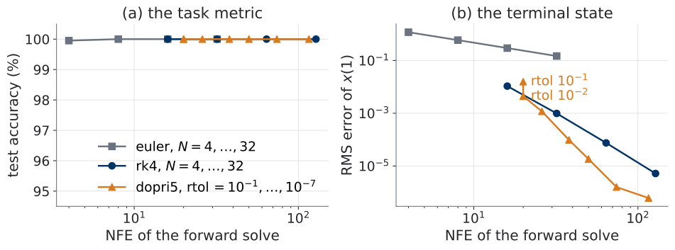
What the two panels say

• Accuracy is 100% in 14 of 15 settings. The exception: Euler, 4 steps, 99.95%.
• The terminal error spans more than 6 decades, from 1.18 down to \(6.1 \times 10^{-7}\).
• At similar cost: rk4, 16 steps, 64 calls, error \(7.5 \times 10^{-5}\); dopri5 at rtol \(= 10^{-6}\), 74 calls, \(1.6 \times 10^{-6}\). Fifth-order adaptive against fixed-step fourth-order: the order alone is not isolated.

On this task, accuracy is nearly blind to solver error: Euler with 4 steps is off by 1.18 in RMS (3.34 at worst) and misses 1 point.

Panel (b) is the ancestor of every quality-against-cost frontier in the course. At the loosest tolerances dopri5 has no advantage over rk4 at the same cost.

NFE against tolerance

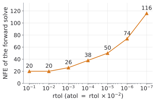
A log-log fit over rtol \(\le 10^{-3}\) gives slope \(-0.16\). It describes this model at this checkpoint, and predicts nothing about the next.

At rtol 1e-1 and 1e-2 the cost is the same; the last decade, 1e-6 to 1e-7, costs 42 more calls.

One step size for the whole batch

torchdiffeq’s controller reduces the error estimate to one number: an RMS over every element of the batched state.

Solve	NFE at the defaults
the 2048 test points, one batch	116
64 of them, both moons, one at a time	50 to 134 (median 74)

60 of 64 points pay more in the batch than alone, and the hardest gets fewer evaluations than it asks for alone. The batch NFE is a property of the batch.

U0.L5 said one step size serves the hardest sample in the batch. Under an RMS norm it does not: the hardest of these points asks for 134 evaluations alone and gets 116 in the batch. A max norm would serve the hardest sample. The tolerance holds for the batch’s RMS error, not for each point. A change of batch composition changes the NFE; U2.L2 will meet it.

TODO 2.3 — NFE across training

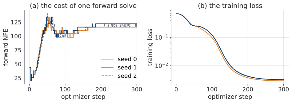
A solver setting fixes a tolerance, not a cost; the cost follows the field.

TODO 2.3 retrains from a fresh initialization with a second seed and logs the forward NFE of each of the first 100 steps of the same schedule. The instruction is to describe, not to confirm: nothing says in advance what the curve does. Board, panel line 3: NFE drift. In the figure, seed 2 is dashed; in the loss panel its curve lies under seed 0’s.

What happened in three runs

• Steps 1–3 cost 44, by arithmetic. The field is still exactly zero (learning rate 0 at step 1; at step 2 the field’s gradient is still zero, so its last layer stays zero), so torchdiffeq’s initial-step rule falls back to \(h = 10^{-6}\), every error estimate is zero, and the step grows by the maximum factor, 10. Seven steps, two start-up calls and six per step: \(2 + 6 \times 7 = 44\).
• Then it falls, and rises. Down to 20 at step 4, the first nonzero field (seed 0); peaks of 134–140 at steps 48–54, while the loss drops from \(\log 2\) to about 0.26; down to 104–110 at step 100, then 116–122 to the end.
• The seeds agree closely. Only the field’s hidden layers are random; both last layers start at zero.

A description of three runs, not a law about Neural ODEs.

Two start-up calls plus six new calls per dopri5 step; the script asserts the 44. Same solver settings throughout: the cost of one forward solve went from 20 at step 4 to 122 at step 300 (seed 0). U2.L2 turns up the gain on this instrument.

04Memory and gradient fidelity

The protocol

torch.cuda.synchronize(); torch.cuda.empty_cache()
torch.cuda.reset_peak_memory_stats()
base = torch.cuda.memory_allocated()
loss = F.cross_entropy(model(x, adjoint=adj,
    method="rk4", options={"step_size": 1 / N}), y)
loss.backward()
torch.cuda.synchronize()
peak = torch.cuda.max_memory_allocated() - base

tracemalloc is not a tensor meter: it sees Python’s allocator, not the native one PyTorch uses. Without a GPU: the process’s resident set size (RSS), sampled, coarse.

Fifty to seventy minutes for the memory and fidelity block, the empirical companion to U2.T1’s two-strategies table. Both routes use fixed-step rk4, so the forward work is identical and only the backward differs. Reset and synchronize around every run, or one run’s peak leaks into the next. Board, panel line 4.

TODO 3.1 — memory against steps

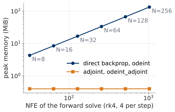
U2.T1’s schematic, with numbers: peak over one forward-and-backward pass. RTX 4070 Laptop GPU, batch 512, float32.

Put U2.T1’s schematic beside it if the projector allows. Same axes; the numbers are the students’.

The reading, and the bill

• Direct backprop: 4.33 MiB at \(N = 8\) to 134.26 MiB at \(N = 256\), about 134 KiB per call.
• Adjoint: 0.40 MiB at every \(N\): constant in the number of steps, for a fixed set of output times. U2.T1’s claim, at its strength.
• The bill: on this fixed grid the adjoint’s backward makes as many field calls as the forward (1024 at \(N = 256\)); direct backprop makes zero. Time: 1.9 times as long at \(N = 8\), 1.6 times at \(N = 256\), here.
• CPU fallback (direct backprop, sampled RSS): tracks the GPU from \(N = 32\) up (127.8 against 134.26 MiB at \(N = 256\)); at \(N = 16\) it read 0.0 MiB against 8.52.

The time ratio is one machine, median of three repetitions, descriptive. The CPU reading shows the trend from N = 32 up and misses the small runs: that is what coarse means. Each adjoint backward call also pays vector-Jacobian products on top of the field.

TODO 3.2 — the fidelity ritual

\(\ell_B\): the loss of the exact flow on a fixed batch \(B\) of 256 test points, the loss of the slide The loss, and what the flow must do with \(\mathcal{D}_{\mathrm{train}}\) replaced by \(B\) (uniform over \(B\)). \(\ell_N\): the same through \(N\) steps of rk4, the loss as the computer evaluates it. Float64; one unit direction \(v\) over the field’s parameters \(\theta_f\); \(\varepsilon = 10^{-6}\).

\[ \begin{aligned} d_{\mathrm{FD}} &= \frac{\ell_N(\theta + \varepsilon v) - \ell_N(\theta - \varepsilon v)}{2\varepsilon}, & d_{\mathrm{AD}} &= v^{\top}\nabla_{\theta_f} \ell_N,\\ d_{\mathrm{ADJ}} &= v^{\top} \hat g_N \ (\text{adjoint's estimate of } \nabla_{\theta_f} \ell_B), & d_{\mathrm{cont}} &= v^{\top}\nabla_{\theta_f} \ell_B \end{aligned} \]

\(d_{\mathrm{cont}}\) is computed two ways that agree to \(1.5 \times 10^{-15}\).

The U0.L1 ritual, unchanged. The finite difference is a witness for the discrete program; direct autodiff is the natural route to the same object. The two routes to d_cont: rk4 with 1024 steps, and dopri5 at rtol 1e-12.

The fidelity table

\(N\)	AD vs FD (rel.)	ADJ vs FD (rel.)	AD vs cont (abs.)	ADJ vs cont (abs.)
8	\(6 \times 10^{-9}\)	\(2 \times 10^{-4}\)	\(1.3 \times 10^{-7}\)	\(8.9 \times 10^{-8}\)
32	\(5 \times 10^{-9}\)	\(3 \times 10^{-6}\)	\(7.8 \times 10^{-10}\)	\(9.6 \times 10^{-11}\)

Relative gaps divide by \(\lvert d_{\mathrm{FD}} \rvert \approx 2.34 \times 10^{-4}\). Absolute gaps to FD: AD \(1.4 \times 10^{-12}\) and \(1.2 \times 10^{-12}\); ADJ \(4.5 \times 10^{-8}\) and \(6.8 \times 10^{-10}\).

• Direct autodiff matches the witness to the order a central difference allows: the exact gradient of the program that ran, as far as the witness can see.
• The adjoint answers a different question, the exact flow’s, discretized.
• Against the exact flow, neither is exact; here the adjoint is closer at both \(N\).

U2.T1’s correctness column, measured: an exact gradient of the wrong function, or an approximate gradient of the right one. The table reports two step sizes; it does not promise the adjoint’s gap falls with N on every problem. Board, panel line 5.

A caution about the ritual’s tolerance

The ritual accepts \(d\) from either route when \(\lvert d - d_{\mathrm{FD}}\rvert \le 10^{-8} + 10^{-6}\max(\lvert d \rvert, \lvert d_{\mathrm{FD}}\rvert)\).

On this trained model the directional derivative is small and the \(10^{-8}\) floor dominates: the adjoint fails at \(N = 8\) and passes at \(N = 32\).

Neither verdict says it is wrong: the ritual catches a wrong gradient, and here its verdict on a legitimate route turns on \(N\). The relative columns separate the routes, and they are well conditioned here: \(|d_{\mathrm{FD}}|\) is eight orders of magnitude above the witness’s own error.

At N = 8 the adjoint fails the ritual; at N = 32 it passes. Neither verdict says the adjoint is wrong.

Margin note — the backward solve can drift

U2.T1: where the forward flow contracts, the backward reconstruction amplifies error. Nothing in the table isolates that effect; on a harder field it is one way the adjoint’s column grows.

Mitigations, named and not oversold:

• tighter tolerances on the backward solve, paid in NFE;
• direct backprop, when the problem is small enough to store;
• checkpointing: store a few states, reconstruct only between them.

The next block shows a library that makes the last one its default.

05The Diffrax mirror

Same classifier, in JAX

The same model in JAX and Diffrax, about thirty lines, loaded with today’s weights. Two checks first, both measured:

• The port agrees with torch: terminal states within \(2.7 \times 10^{-13}\) at a tight tolerance.
• Diffrax reports steps, not calls; a jax.debug.callback counts 49 calls for 8 steps of Dopri5: six per step, one at the start.

Two of the routes behind one argument, adjoint=: RecursiveCheckpointAdjoint (the default) and BacksolveAdjoint.

Seventy to eighty-five minutes for the Diffrax block: if time is short it goes home whole, and it is self-contained. Second of the three joint labs that use JAX (U1.L1, here, U3.L1).

TODO 4.1 — honest timing

Adjoint	\(N\)	trace + lower + compile	steady, per call
RecursiveCheckpointAdjoint	8	1.43 s	9.3 ms
BacksolveAdjoint	8	1.68 s	8.0 ms
RecursiveCheckpointAdjoint	32	1.40 s	42.1 ms
BacksolveAdjoint	32	1.55 s	31.9 ms

Value and gradient, 256 points, float64, Intel Core Ultra 9 185H CPU, one run. The up-front price is the whole first-call overhead; at \(N = 8\) it equals about 153 steady calls of the checkpointed route. Do not rank frameworks with this table.

The U0.L5 rule: the up-front price (tracing, lowering, compilation) apart from steady state, always. Tracing and lowering are the larger part of it here. The nearest torch call, direct backprop through rk4 with 8 steps, took 9.5 ms on the same machine, but solver, tableau, compiler and threads all differ. Board, panel line 6.

TODO 4.2 — two philosophies, one metric

\(N\)	RecursiveCheckpointAdjoint vs FD	BacksolveAdjoint vs FD
8	\(2.1 \times 10^{-8}\)	\(3.4 \times 10^{-5}\)
32	\(3.8 \times 10^{-10}\)	\(2.7 \times 10^{-8}\)

Relative gaps, same direction \(v\), same batch, fixed-step Dopri5.

• Checkpointed: discretize, then optimize. Agrees with its own program.
• Backsolve: optimize, then discretize; the continuous adjoint of U2.T1. Diffrax’s documentation marks it “not recommended” (Kidger 2021).
• The ritual’s verdict passes both routes at both \(N\); only the size of the gaps tells them apart.

The point is not that one keyword reproduces the torch trade exactly. The API puts the two philosophies side by side, and the metric tells them apart.

Two libraries, two emphases

• Diffrax defaults to checkpointed backpropagation.
• torchdiffeq still exposes the classical continuous adjoint as its prominent memory-saving route; there the route is the function you call, odeint or odeint_adjoint.

Neither is wrong; they weigh one trade differently. Know which route you run before you read “we trained with the adjoint”.

The numerics behind Diffrax’s defaults: Kidger (2022, ch. 5), optional.

Research literacy: the default of the library a paper used is part of its method.

06The instrument panel

The panel

Instrument	What it read today
NFE counter	every call, forward and backward
NFE-vs-quality axes	accuracy flat; error across 6 decades
NFE drift in training	20 at step 4, 122 at step 300
Peak-memory protocol	direct grows; the adjoint stays flat
Gradient-fidelity table	two routes, two different numbers
Honest timing	compile apart from steady state

Every gauge on this panel gets pointed at a generative model in the FFJORD lab — and there, the needles move. Watch them.

Eighty-five to ninety minutes. Read the board’s panel, line by line; it should match this slide. Then the closing sentence, verbatim. The corner question from U2.T1 stays where it is.

What comes next

• Next session (U2.T2): back to the question U2.T1 left on the board.
• The lab after it (U2.L2): today’s instruments, on the model that question leads to.
• The solutions notebook is released today.

Sources for today: torchdiffeq (Chen 2018), Diffrax (Kidger 2021), the Neural ODE paper (Chen et al. 2018, sec. 2), and Massaroli et al. (2020, App. A.1).

Two sentences and out.

References

Chen, Ricky T. Q. 2018. “torchdiffeq: ODE Solvers and Adjoint Sensitivity Analysis in PyTorch.” https://github.com/rtqichen/torchdiffeq.

Chen, Ricky T. Q., Yulia Rubanova, Jesse Bettencourt, and David Duvenaud. 2018. “Neural Ordinary Differential Equations.” In Advances in Neural Information Processing Systems. https://arxiv.org/abs/1806.07366.

Kidger, Patrick. 2021. “Diffrax: Numerical Differential Equation Solvers in JAX.” https://github.com/patrick-kidger/diffrax.

———. 2022. “On Neural Differential Equations.” PhD thesis, University of Oxford. https://arxiv.org/abs/2202.02435.

Massaroli, Stefano, Michael Poli, Jinkyoo Park, Atsushi Yamashita, and Hajime Asama. 2020. “Dissecting Neural ODEs.” In Advances in Neural Information Processing Systems. https://arxiv.org/abs/2002.08071.