U1.T2 — The Zoo and Its Limits

Flow-Based Generative Models · UFRJ · 2026.2

01Glow: the coupling family at image scale

Three debts, on the board

Left open	By	Paid in
The depth question — how expressive is a stack of coupling layers?	U1.T1	the universality block
The fine print — a flow is a diffeomorphism; what can one not do?	U1.T1	the topology block
The checkerboard gaps — \(29.8\%\) of the mass where the data density is zero	U1.L1	the topology block

Before the debts: the rest of the zoo (the Glow and autoregressive blocks), read through one table.

Zero to two minutes. BOARD 1 is U1.T1’s two-costs table, redrawn with the two rows and empty space under them. BOARD 2 carries the three debts as written here. Say the joint-audience sentence once: this session depends on U1.T1, U1.L1 and UP.T1, and on nothing from the bootcamp. The one bootcamp callback, the autoregressive factorization, is on the slide in full when it comes.

The two costs, version 1

Operation	Direction	Needs, per layer	Cost driver
Sampling	forward, \(z \to x\)	evaluate \(\psi_k\)	one pass per layer
Density / training	inverse, \(x \to z\)	\(\psi_k^{-1}\) and \(\log\lvert\det J_{\psi_k}\rvert\)	the inverse, and the log-det

The unit’s thesis: the zoo is a list of tricks to make both rows cheap at once.

Today the table gets one row per family (v2). Convention unchanged: \(\psi \colon z \to x\) generates; a library’s \(f \colon x \to z\) is \(f = \psi^{-1}\). U1.T1 wrote the same two rows as \(x_0 \to x_1\) and \(x_1 \to x_0\); these are U1.L1’s letters.

Two to four minutes. Point at the empty space under the two rows. Every family today is placed there, and the block-G slide is what the board looks like at the end. Say the direction convention once and never again.

Glow is RealNVP, engineered

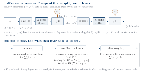
Affine coupling at \(32 \times 32\) and \(256 \times 256\) (Kingma and Dhariwal 2018, sec. 3), with two extra layer types whose log-determinants are as cheap as coupling’s:

• actnorm: a per-channel scale and bias, in place of batch normalization;
• invertible \(1 \times 1\) convolution: a learned permutation of the channels;

and a multi-scale arrangement of the stack. No new theorem.

Four to five minutes. The claim to land: nothing in block A changes what block D will say. Glow lives entirely in the coupling row.

Actnorm

On an \(h \times w \times c\) feature map, with \(s, b \in \mathbb{R}^{c}\), at every position \((i, j)\):

\[ \begin{aligned} y_{ij} &= s \odot x_{ij} + b, \qquad x_{ij} = (y_{ij} - b)/s, \\ \log\lvert\det J\rvert &= h\,w \sum_{j=1}^{c} \log\lvert s_j\rvert . \end{aligned} \]

Example, a \(32 \times 32 \times 12\) map: \(24\) parameters; \(\log\lvert\det J\rvert = 1024 \sum_{j=1}^{12} \log\lvert s_j\rvert\) — twelve logarithms, one sum.

Five to seven minutes. The diagonal Jacobian with each scale repeated hw times; write the sum on the board.

Actnorm is not batch normalization

• \(s, b\) are initialized from the first minibatch: zero mean, unit variance per channel (Kingma and Dhariwal 2018, sec. 3.1).
• After that they are ordinary parameters: no batch statistics, no train/eval split, one function of one input.
• Invertible when every \(s_j \neq 0\).

Data-dependent initialization chooses the starting point. It is not a normalization layer.

The one sentence that matters is on the slide: data-dependent initialization is a way to choose the starting point, not a normalization layer.

The invertible \(1 \times 1\) convolution

One matrix \(W \in \mathbb{R}^{c \times c}\) at every position; a permutation is the case \(W = P\):

\[ \begin{aligned} y_{ij} &= W x_{ij}, \qquad \log\lvert\det J\rvert = h\,w\,\log\lvert\det W\rvert \\ &= h\,w \sum_{i=1}^{c} \log\lvert s_i\rvert \quad\text{for } W = P L (U + \operatorname{diag} s). \end{aligned} \]

• \(P\) fixed permutation, \(L\) unit lower-triangular, \(U\) strictly upper, \(s\) learned (Kingma and Dhariwal 2018, sec. 3.2). Invertible when every \(s_i \neq 0\).
• Determinant bookkeeping: \(O(c)\). Applying the mixing: still \(O(h w c^{2})\).
• Same \(32 \times 32 \times 12\) map: \(144\) parameters, \(1024 \times 144\) multiply-adds to apply, twelve logarithms for the log-det.

Seven to nine minutes. Say the cost sentence exactly: PLU makes the determinant cheap, not the convolution. The dense channel mixing is the price of learning the permutation.

Multi-scale, in one picture

Nine to eleven minutes. Read the top row left to right in the density direction; say that sampling runs the arrows backwards. Squeeze is a reshape, log-det zero. Split is a partition of the state, not a transform. U1.L2 makes this executable; today it is a picture.

Glow on the table

	Density / likelihood	Sampling
Glow	exact: coupling sums \(+\) actnorm sums \(+\) PLU sums	direct: every layer has an analytic inverse

The coupling row, engineered for images. It removes no limitation that the universality and topology blocks will state.

Eleven to twelve minutes. Write the Glow row on BOARD 1. Then turn the page: the next family is where the two costs come apart.

02Autoregressive flows: MAF and IAF

The autoregressive factorization

Any density on \(\mathbb{R}^{d}\) factorizes by the chain rule. With coordinates \(x = (\xi_1, \dots, \xi_d)\):

\[ p(x) = \prod_{i=1}^{d} p(\xi_i \mid \xi_{<i}), \qquad \xi_{<i} = (\xi_1, \dots, \xi_{i-1}). \]

A network that produces each factor from earlier coordinates only has an exact likelihood and a fixed ordering. That is the whole autoregressive (AR) family.

Coordinates are \(\xi_i\) (of \(x\)) and \(\zeta_i\) (of \(z\)): in this course \(x_1\) is a data point, never a coordinate.

Twelve to fourteen minutes. Self-contained on the slide by the parity rule; PGMAT hears U0.T3’s panorama, PESC reads a definition. The coordinate letters are a course convention and are worth ten seconds.

MAF: the density transform

Parameterize \(f = \psi^{-1} \colon x \to z\) coordinate by coordinate (Papamakarios, Pavlakou, and Murray 2017, sec. 3):

\[ \zeta_i = \frac{\xi_i - \mu_i(\xi_{<i})}{\sigma_i(\xi_{<i})}, \qquad \log\lvert\det J_{\psi}(z)\rvert = \sum_{i=1}^{d} \log\sigma_i(\xi_{<i}) . \]

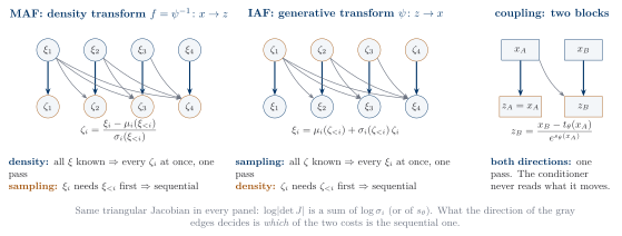
• Density: one pass. Every \(\xi_i\) is known, so one masked network (its masks let output \(i\) read only \(\xi_{<i}\)) gives all \((\mu_i, \sigma_i)\) at once.
• Sampling: sequential. \(\xi_i = \mu_i(\xi_{<i}) + \sigma_i(\xi_{<i})\,\zeta_i\) needs \(\xi_{<i}\) first.

Fourteen to seventeen minutes. Write the density transform on the board and the inverse recursion under it. Say “the conditioner reads the data coordinates” and underline “data”.

IAF: the generative transform

Parameterize \(\psi \colon z \to x\) instead, with the conditioner reading the source coordinates (Kingma et al. 2016, secs. 3–4):

\[ \xi_i = \mu_i(\zeta_{<i}) + \sigma_i(\zeta_{<i})\,\zeta_i, \qquad \log\lvert\det J_{\psi}(z)\rvert = \sum_{i=1}^{d} \log\sigma_i(\zeta_{<i}) . \]

• Sampling: one pass. Every \(\zeta_i\) is known.
• Density: sequential. \(\zeta_i = (\xi_i - \mu_i(\zeta_{<i})) / \sigma_i(\zeta_{<i})\) needs \(\zeta_{<i}\) first.

Seventeen to nineteen minutes. Same shape, other side. Underline “source”. Do not yet say “duality”; let the next slide say it carefully.

Duality: the direction of a triangle

Nineteen to twenty-two minutes. The named asset of the session. Read the gray edges: in MAF they leave the data row, in IAF they leave the source row. Say the sentence the L3 insists on: these are different parameterized families with opposite dependency directions, not the same map read backwards. And point at the right panel: coupling is the two-block version, and the conditioner never reads what it moves — which is why both of its directions are one pass, and why it needed depth and permutations.

MAF and IAF on the table

Family	Density / likelihood	Sampling
MAF	parallel, one pass	sequential inverse (event dimension)
IAF	sequential inverse (event dimension)	parallel, one pass

“\(d\) passes” is an intuition for affine scalar autoregression. The implementation-level statement is sequential in the event dimension — along the \(d\) coordinates of one point — not a promise about a count of network calls.

Twenty-two to twenty-four minutes. Two rows on BOARD 1. The “d passes” calibration is one sentence and worth saying, because the phrase will appear in seminar papers with a precise-sounding count that depends on caching.

Coupling is block-autoregressive

Two blocks in place of \(d\) coordinates: \(z_A = x_A\) copied, \(z_B = (x_B - t_\theta(x_A)) \odot e^{-s_\theta(x_A)}\) conditioned on the first.

• U1.T1’s affine coupling layer is an autoregressive map with two blocks (Papamakarios et al. 2021, sec. 3.1.2).
• The conditioner never reads what it moves, so both directions are one pass.
• The price: one coupling layer cannot represent an arbitrary autoregressive map. Expressivity is paid in depth, with permutations between layers (U1.T1 §6).

Coupling, MAF and IAF: one triangular idea, at different block sizes, in different directions.

Twenty-four to twenty-six minutes. The zoo is unified here, and the depth question of block C is set up by the third bullet.

03Universality, and its fine print

The depth question, first half: a negative result

NICE’s additive layers, and any stack of them, are volume-preserving: \(\lvert\det J\rvert = 1\).

Flows with constant Jacobian determinant are not universal distribution approximators under KL. A flow of constant-Jacobian diffeomorphisms has the same number of modes as its base distribution.

A constant factor on the density cannot move a maximum. NICE’s final scaling layer does not help: its determinant is a constant, so the theorem applies with the layer as without it — the answer to U1.T1’s Exercise 2. What removes the obstruction is a determinant that varies with the input: RealNVP’s \(e^{s_\theta(x_A)}\) (Draxler et al. 2024, sec. 4).

Twenty-six to twenty-eight minutes. The mode-count sentence is the memorable one. U1.T1 said additive coupling cannot change local volume and deferred the scaling-layer question to today; the answer is that a constant determinant, scaled or not, is what the theorem is about.

The depth question, second half: a positive result

Constant-Jacobian stacks are capped. Does depth in a richer family do better? Yes, with fine print:

For every continuous density \(p\) on \(\mathbb{R}^{d}\) with finite first and second moments and infinite support, there is a sequence of flows \(f_n\) of \(n\) affine coupling blocks, each \(L\)-bi-Lipschitz (distances stretched or compressed by at most a factor \(L\), in either direction), with \((f_n)_{\#}\,p \to \mathcal{N}(0, I_d)\) as \(n \to \infty\) — in the paper’s convergence measure \(\Delta_{\text{affine}}\) (the KL improvement one more block could buy), which KL-convergence implies.

Twenty-eight to thirty minutes. Read the three hypotheses out loud, slowly, and underline “infinite support”. The convergence is in the paper’s own measure; KL convergence is what they observe and conjecture. Say that, because the fine-print slide is two slides away.

Why the affine case needed its own theorem

The classical argument (Papamakarios et al. 2021, sec. 2.2, §3.1.2):

• For any everywhere-positive target with differentiable conditional CDFs, the conditional-CDF map \(\zeta_i = \Pr(\xi_i' \le \xi_i \mid \xi_{<i})\) is a triangular diffeomorphism onto the uniform on \((0,1)^{d}\).
• An autoregressive flow represents it when conditioners and transformers are flexible enough; \(d\) coupling layers with the right splits represent any autoregressive map.
• An affine transformer is not flexible enough: for fixed \(\xi_{<i}\) it is affine in \(\xi_i\), and an affine function is not a conditional CDF.

So the classical existence argument says nothing about RealNVP. The theorem on the previous slide is what settles the affine case.

Thirty to thirty-one minutes. One slide, so that nobody leaves believing the CDF construction already covered coupling flows. The survey itself says the classical argument “makes no guarantees about the flow’s behavior in practice”.

The fine print, read slowly

1. Existence over a growing family. For each \(n\) a good flow exists; nothing says training finds it, and no bound on \(n\) is given.
2. The hypotheses on the target matter. Continuity, finite moments, infinite support. The gapped checkerboard fails two of three.
3. Nothing about finite depth, trainability, or the conditioning of the composition. Blocks are \(L\)-bi-Lipschitz; the stack is not bounded independently of \(n\).
4. Approximating a distribution is not approximating a map. Many maps push \(p_0\) near the same target.

Thirty-one to thirty-three minutes. Item 2 is the pivot and item 3 is block D’s second half. Then ask the question of the next slide out loud.

The pivot

Universality holds, with fine print, for targets of infinite support.

What happens when the target has literal hard-zero gaps — a support in several pieces — that a flow from a Gaussian source cannot reproduce exactly?

That is the checkerboard. The answer is a theorem about supports.

Thirty-three to thirty-four minutes. Turn to BOARD 2. Write “support, not level sets” at the top and leave it there for the whole of block D.

04Exact support: the topology obstruction

Replay: the gapped checkerboard

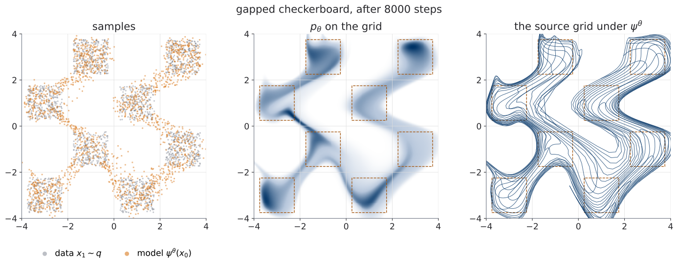
Eight separated squares, exactly zero density between them; \(0\) of \(100{,}000\) generated points outside. The model: \(29.8\%\) of its mass in the gaps, NLL \(0.50\) nats above \(\log 18\).

Thirty-four to thirty-six minutes. U1.L1’s figure, unchanged. The dataset contract matters for everything that follows: hard gaps, no jitter. The lab recorded four numbers and explained none; by the end of the block each has a status.

The precision rule

“Topology obstruction” is a statement about supports and globally invertible maps.

It is not a statement about density level sets. A diffeomorphism can make a bimodal density from a unimodal source — U1.L1’s two-moons model is the proof by example.

Recall: the support of \(P\) is the closed set of points all of whose open neighbourhoods have positive measure. \(\operatorname{supp}\mathcal{N}(0, I_d) = \mathbb{R}^{d}\). The checkerboard’s support is eight closed squares: disconnected.

Thirty-six to thirty-seven minutes. This slide exists so that nobody leaves with “flows preserve topology” as a sentence about modes. Point at the board: support, not level sets.

The support proposition

Let \(P\) have support \(S\) and let \(\psi \colon \mathbb{R}^{d} \to \mathbb{R}^{d}\) be a homeomorphism (onto, continuous, continuous inverse). Then \[ \operatorname{supp}(\psi_{\#}P) = \psi(S). \] If \(S\) is connected, so is the support of the pushforward.

Proof. (\(\supseteq\)) \(V\) open around \(\psi(s)\), \(s \in S\): \(\psi^{-1}(V)\) is open around \(s\), so \(P(\psi^{-1}(V)) > 0\).
(\(\subseteq\)) \(y\) in the support, \(s = \psi^{-1}(y)\), \(U\) open around \(s\): \(\psi(U)\) is open around \(y\), so \(P(U) = \psi_{\#}P(\psi(U)) > 0\), hence \(s \in S\). Connectedness: continuous image of a connected set. \(\blacksquare\)

Thirty-seven to forty-one minutes. Live, on BOARD 2, both inclusions; each is two lines and the second uses that psi is onto and open. Say where the closure would enter if psi were only onto an open subset (the notes’ remark), and that every architecture of the unit is onto, so it does not.

Every flow of this unit is onto \(\mathbb{R}^{d}\)

Layer	Why it is a bijection of \(\mathbb{R}^{d}\) onto \(\mathbb{R}^{d}\)
affine coupling	analytic inverse, defined for every \(x\)
actnorm, \(1 \times 1\) conv	affine and linear, \(s_j \neq 0\), \(\det W \neq 0\)
MAF, IAF, \(\sigma_i > 0\)	inverse recursion: one affine equation per coordinate
permutation, squeeze	reshapes and swaps
residual, \(\operatorname{Lip}(g) < 1\)	\(x + g(x) = z\) has one solution (residual-flow block)

\[ \operatorname{supp} p_\theta = \psi^{\theta}(\mathbb{R}^{d}) = \mathbb{R}^{d} \qquad\text{for every } \theta . \]

Forty-one to forty-two minutes. The residual row is a promissory note paid in block E. The formula is the verdict; the next slide reads it.

The verdict, and what it is not

A flow of this unit cannot exactly equal:

1. a target whose support is disconnected — the checkerboard: \(\mathbb{R}^{2}\) is not eight squares, for any \(\theta\);
2. a target whose support has empty interior — a distribution on a curve or a surface.

Not capacity, not depth, not optimization.

Not about level sets. The model’s superlevel sets \(\{p_\theta > c\}\) can be disconnected: \(\lvert\det J\rvert\) varies from point to point. A constant Jacobian guarantees the mode count (the universality block); a variable one guarantees nothing, and two-moons shows the count changing. Do not write “level-set topology is preserved” — it is false.

Forty-two to forty-four minutes. Item 2 is the one-line U6 pointer: manifold data wants a source and a domain that live on the right space. Then the level-set paragraph, said once more, because it is the sentence students get wrong.

Approaching a mismatched target

The proposition rules out equality. What does closeness cost? Define the bi-Lipschitz constant \[ \begin{aligned} \operatorname{BiLip}(f) = \inf\Big\{ M \in [1, \infty] :\ & M^{-1}\lVert z - z'\rVert \le \lVert f(z) - f(z')\rVert \\ & \qquad \le M \lVert z - z'\rVert \ \text{ for all } z, z' \Big\}. \end{aligned} \]

\(\operatorname{BiLip}(f) = \infty\) when no finite \(M\) works. A large constant means that somewhere the map stretches or compresses enormously, and its inverse does the opposite: the constant measures how numerically invertible \(f\) is.

Forty-four to forty-six minutes, with the theorem slide.

Cornish’s theorem

If \(\operatorname{supp} P_Z\) and \(\operatorname{supp} P^{\star}\) are not homeomorphic, then for any measurable \(f_n\): \[ (f_n)_{\#}P_Z \to P^{\star} \ \text{weakly} \quad\Longrightarrow\quad \operatorname{BiLip}(f_n) \to \infty . \]

Weak convergence — expectations of bounded continuous functions converge — is implied by minimizing KL. So: approaching the checkerboard forces the flow to become arbitrarily badly conditioned (Cornish et al. 2020, sec. 2).

Stated, not proved; the proof is the paper’s supplement B.3. Say what “not homeomorphic” is here: R^2 connected, eight squares not.

Cornish’s corollary, and who pays first

Corollary 2.2. For any weak-topology metric \(\rho\) there is \(M(\varepsilon) \to \infty\) as \(\varepsilon \to 0\) such that: target within \(\varepsilon\) of a mismatched \(P^{\star}\), model within \(\varepsilon\) of the target \(\Rightarrow\) \(\operatorname{BiLip}(f) \ge M(\varepsilon)\).

• The realistic case: a nearly hard-gapped target costs almost as much as a hard-gapped one.
• Universality says the approximation exists; this says what it costs.
• A residual flow of \(K\) blocks with \(\operatorname{Lip}(g_k) \le \kappa < 1\) has \(\operatorname{BiLip} \le \max(1 + \kappa, (1 - \kappa)^{-1})^{K}\) (Cornish et al. 2020, eq. 6): bounded by construction, against a theorem that demands unbounded.

Forty-six to forty-eight minutes. The third bullet is the bridge to block E: the very condition that makes residual flows invertible is the one that caps their bi-Lipschitz constant. Coupling flows have no such a-priori cap, which is not the same as being well-conditioned.

The price of a gap, in closed form

Forty-eight to fifty minutes. One dimension: source N(0,1), target a Gaussian bulk times epsilon on the gap; support R for every epsilon > 0, so the proposition does NOT apply and exact equality IS possible. The unique increasing map is the quantile transform, and its slope is the change of variables read backwards: small target density, large slope. Panel (c): Lip times gap mass stays between 0.412 and 0.414 for every epsilon <= 0.3; halve the bridge, double the steepness; the inverse direction never exceeds 0.86. Say clearly that this is one family in one dimension, computed, and not a theorem about d = 2 or about trained models.

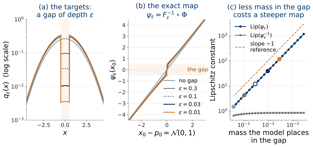
The price of a gap, as a sweep

The same family, as a sweep from epsilon = 1 to 0.01, with every number computed at the frame. At epsilon = 1 the map is the straight line 1.5 x0: the 1.50 is a slope everywhere, not yet a price. From epsilon <= 0.3 the largest slope sits at the gap edge (orange dot): 12.1 at 0.1, 118 at 0.01, while the inverse stays at or below 0.850. The last frame draws epsilon = 0 dashed, as a separate object: a jump at x0 = 0, no longer a homeomorphism, and the support proposition takes over.

Reading the checkerboard correctly

Observation on a trained flow	Status
nonzero model density in hard-zero gaps	structural (full-support source \(+\) diffeomorphism)
extreme Jacobian conditioning as the mismatch is pushed	supported by the theorem
inverse round-trip degradation, instability	plausible numerical consequence; measure it
NLL plateau, poor samples	non-specific: capacity or optimization

Fifty to fifty-two minutes. Give each of U1.L1’s four numbers its row. This table comes back in U7.W1 as a debugging aid; say so.

What \(29.8\%\) is a number about

• Structural: every finite, regular, Gaussian-based flow puts nonzero density in the gaps.
• Not structural: the amount. \(29.8\%\) is a fact about one six-layer model, trained 8000 steps at a bounded log-scale — not about diffeomorphisms.
• The bridge can be pushed toward zero; the price is conditioning (the theorem, and the one-dimensional family).
• The half nat above \(\log 18\) is \(\mathrm{KL}(q \,\Vert\, p_\theta)\): never exactly zero for a flow of this unit, but with no positive floor — it can be driven toward zero at the conditioning cost. \(0.50\) is what this architecture paid.

Topology is a hypothesis to test, not a verdict every bridge proves.

Fifty-two to fifty-three minutes. The calibration sentence, said in full. A deeper model or a relaxed scale bound would put less mass in the gaps and pay in conditioning.

Where the obstruction goes next

• U2. A flow of a well-posed differential equation is still a diffeomorphism of \(\mathbb{R}^{d}\) onto itself. Continuous time changes the parameterization and the costs, not this constraint. U2 adds a separate restriction of its own; the two stay apart.
• U3. A hard-support target forces a choice at the data end of the path from \(p_0\) to \(q\): a limiting endpoint, or a smoothed one.
• U6. Manifold data: choose a source and a map that live on the right space; on that space a regular flow is still a diffeomorphism, and the proposition applies unchanged.

Fifty-three to fifty-four minutes. Three pointers, one line each. Do not open any of them.

05Residual flows: invertibility without triangularity

The dialect, declared once

Everything so far bought a cheap log-det by forcing a triangular Jacobian. Residual flows give that up.

The literature writes the map the way a residual network computes it — data to source. That is the density transform:

\[ f = \psi^{-1}, \qquad f(x) = x + g(x), \qquad g \colon \mathbb{R}^{d} \to \mathbb{R}^{d} \text{ a network}. \]

The identity plus a perturbation. If the perturbation is small enough, the identity wins. “Small enough” is a Lipschitz condition (Behrmann et al. 2019, sec. 2).

Fifty-four to fifty-six minutes. BOARD 3 opens. Say the convention once: psi still generates; f is the letter for its inverse, as U1.T1’s library note allowed.

Invertibility by Banach

Fix \(z\); \(x + g(x) = z\) is the fixed-point equation \(x = z - g(x)\). Iterate: \[ x^{(m+1)} = z - g\big(x^{(m)}\big), \qquad x^{(0)} = z . \]

If \(\operatorname{Lip}(g) = L < 1\), then \(T_z(x) = z - g(x)\) satisfies \[ \lVert T_z(x) - T_z(x')\rVert = \lVert g(x') - g(x)\rVert \le L\,\lVert x - x'\rVert . \]

Banach on the complete space \(\mathbb{R}^{d}\): a unique fixed point, hence a unique solution of \(f(x) = z\) — \(f\) is a bijection of \(\mathbb{R}^{d}\) onto itself, and the iteration converges to \(f^{-1}(z)\) from anywhere (Behrmann et al. 2019, Thm. 1). On the Measured, on one block slide: \(L = 0.5\) reaches \(10^{-10}\) in \(27\) iterations; \(L = 0.95\) has not after \(60\).

Fifty-six to fifty-nine minutes. The two lines, live, on BOARD 3; the second line is the definition of L. Then say “Banach” and stop: the rest is PS1.5. Pay the promissory note from block D: the residual row of the “onto” table is this slide.

PS1.5 — residual-flow invertibility via Banach

With \(\operatorname{Lip}(g) = L < 1\) and \(f(x) = x + g(x)\):

• (a) \(T_z(x) = z - g(x)\) is an \(L\)-contraction, with the definitions written out.
• (b) Banach on \(\mathbb{R}^{d}\) (say why it is complete): \(f\) is a bijection of \(\mathbb{R}^{d}\) onto itself and the iteration converges to \(f^{-1}(z)\) from every start.
• (c) \(\operatorname{Lip}(f) \le 1 + L\) and \(\operatorname{Lip}(f^{-1}) \le 1/(1 - L)\): \(f\) is a homeomorphism, and a diffeomorphism when \(g\) is \(C^{1}\).
• (d) Bonus. \(\lVert x^{(m)} - x^{\ast}\rVert \le L^{m}(1 - L)^{-1}\lVert x^{(1)} - x^{(0)}\rVert\); iterations for tolerance \(\delta\); the cost of one sample from \(K\) blocks.

Enforcing \(L < 1\): spectral normalization — divide each weight matrix by (a bound on) its largest singular value (Behrmann et al. 2019, sec. 2.1). This is the bounded constant of the topology block.

Fifty-nine to sixty-one minutes. Assign and move on. Part (c) is the bound Cornish’s eq. 6 is built from. Part (d) is the dashed line on the Measured, on one block slide.

The log-determinant, as a series

\(J_f = I + J_g\) is dense. Under \(\lVert J_g\rVert_2 \le L < 1\): every eigenvalue of \(J_f\) has positive real part, so \(\det J_f > 0\); and \(\log\det = \operatorname{tr}\log\) has a power series:

\[ \begin{aligned} \log\det\big(I + J_g\big) &= \sum_{k=1}^{\infty} \frac{(-1)^{k+1}}{k}\,\operatorname{tr}\big(J_g^{k}\big), \\ &\qquad \text{valid when } \rho(J_g) < 1 . \end{aligned} \]

The condition is part of the formula — the Maclaurin series of \(\log(1 + a)\) with a matrix for \(a\), convergent for the same reason. Truncation after \(n\) terms: error \(\le d \sum_{k > n} L^{k}/k\), geometric at rate \(L\) (Behrmann et al. 2019, sec. 3, Thm. 3).

Sixty-one to sixty-four minutes. Write the series with its condition on BOARD 3 and box the condition. Do not present it as algebra valid for any matrix; for a block that is not contractive the right-hand side diverges.

Hutchinson’s estimator

Infinitely many traces of matrices that are never formed. The device:

For \(A \in \mathbb{R}^{d \times d}\) and a random \(v\) with \(\mathbb{E}_{v}[v v^{\top}] = I_d\) (Rademacher \(\pm 1\), or Gaussian): \[ \operatorname{tr}(A) = \mathbb{E}_{v}\big[\, v^{\top} A\, v \,\big]. \]

Usage. \(v^{\top} J_g^{k} v\) by \(k\) vector–Jacobian products: \(w^{\top} \leftarrow v^{\top}\), then \(w^{\top} \leftarrow w^{\top} J_g\) \(k\) times, then \(w^{\top} v\). One backward pass of \(g\) per product; \(J_g\) never materialized. One probe serves every term.

Deferred. Proof and variance: U2.T2, where the estimator carries the weight. Named only: the truncated series is biased; the Russian-roulette estimator of (Chen et al. 2019) removes the bias by a random truncation with reweighting.

Sixty-four to sixty-seven minutes. State and use; do not prove. The E_v subscript stays. Russian roulette is a name today and a mechanism never, in this unit.

Measured, on one block

Sixty-seven to seventy minutes. One block in d = 6 with Lipschitz constant exactly L, three values. (a) The iteration under the Banach bound: L = 0.5 hits 1e-10 in 27 steps; L = 0.95 has not after 60. (b) The series truncation: 1e-6 needs 15, 40 and 146 terms. (c) Hutchinson on the L = 0.8 block: the 5–95% envelope over 200 probe streams closes on the exact trace 2.865; the grand mean is 1.1 standard errors from the truth (asserted within four); the spread is 0.057 at 100 probes, 0.0055 at 10,000. Everything asserted by the script.

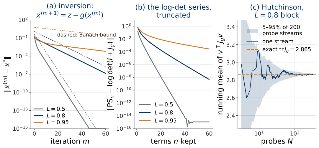
Residual flows on the table

	Density / likelihood	Sampling
Residual flow	\(f(x) = x + g(x)\) direct; \(\log\lvert\det J\rvert\) an infinite series, estimated stochastically	\(\psi = f^{-1}\) by fixed-point iteration, several evaluations of \(g\) per block

One row stochastic and approximate, the other iterative and exact to any tolerance. Not “both directions are stochastic”.

Seventy to seventy-two minutes. The last row on BOARD 1. Say the correction in the last line out loud: sampling is exact to tolerance, at the cost of iterations.

06Depth to infinity: the cliffhanger

A residual stack with a step size

Put a step \(h = 1/K\) in front of each residual branch and let the branch depend on a time \(t_k = k h\):

\[ x_{k+1} = x_k + h\,f(t_k, x_k), \qquad k = 0, \dots, K-1 . \]

The letter \(f\) is now the right-hand side of a differential equation, time first — the course’s f(t, x); the residual branch of the residual-flow block is \(g_k = h f(t_k, \cdot)\). This is the forward-Euler step, and as \(h \to 0\) the stack’s output converges, for a regular enough \(f\), to the solution of \[ \frac{\mathrm{d}x}{\mathrm{d}t} = f(t, x), \qquad t \in [0, 1] . \]

Seventy-two to seventy-four minutes. BOARD 3, under the series: the Euler rewrite. Say the letter change out loud. Nothing continuous is derived from here to the end.

Measured: the stack converges as \(h \to 0\)

Seventy-four to seventy-seven minutes. (a) K = 4, 16, 64 against a high-accuracy reference. (b) Halving h halves the endpoint error, from 0.60 at K = 2 to 0.0012 at K = 1024, every ratio between 1.91 and 2.03. (c) The grid under the 64-step stack: one sheet. The field is Lipschitz on the whole plane (a damped pull; a cubic one would not be, and then no step would make the block a contraction everywhere), so each Euler block has residual branch h f with h Lip(f) <= 0.041 < 1 and is a residual-flow block in block E’s sense on all of R^2; the stack is inverted block by block to 1e-15. Blocks D, E and F in one panel.

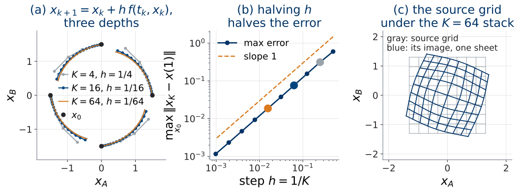
The stack, one doubling at a time

Panel (a) as a sequence: the same four starting points, K doubling from 2 to 256. Every segment splits at its midpoint and the new vertices move; the gray curves never move, only K changes. For the drawn points the max endpoint error goes from 0.6014 to 0.0047, every ratio between 1.91 and 2.03. The last frame is the question the next slides leave open: the log-det is a sum of K terms; what does it become?

The promise, without overclaiming

• Discrete residual invertibility needed a strong layerwise condition: every block a contraction. That capped the bi-Lipschitz constant (the topology block) and is what spectral normalization enforces.
• A well-posed equation is invertible on its interval under existence-and-uniqueness and no-blow-up conditions: run it backwards. The field still needs regularity — a Lipschitz-type assumption does not disappear — but the architecture is no longer forced to make every finite block a contraction.
• The stack’s log-det is \(\sum_k \log\det(I + h J_f)\). As \(h \to 0\) it wants to become an integral. What it becomes is not derived here.

Seventy-seven to eighty minutes. Three bullets, each with its qualifier, so that U2 can be held to them. The third is the cliffhanger.

Left on the board for U2

What does \(\log\lvert\det J\rvert\) become in continuous time?

Not answered today. U2.T1 sets up the flows of differential equations and the cost of a solver inside every training step; U2.T2 answers this question, with Hutchinson’s estimator on the critical path.

Eighty to eighty-one minutes. Write the question top-right on BOARD 3 and do not erase it. U2.T1 rewrites it at minute zero.

07Unit close: the two costs, version 2

The two costs, version 2

Family	Density	Sampling	Trick, and its price
NICE / RealNVP	exact, triangular	direct	coupling; depth
Glow	exact	direct	mixing, multi-scale
MAF	parallel	sequential	AR, data side
IAF	sequential	parallel	AR, source side
Residual flow	direct; series log-det	iterative	contraction, traces

Version 3 in U2.T2, where the cells change. U3.L1 touches neither column.

Eighty-one to eighty-four minutes. This is BOARD 1 as it stands. Read it once, top to bottom.

Reading the unit

• Exactness was achieved in U1.T1, by construction.
• Architecture choices expose computational dualities: a triangle read in either direction; the direction decides which cost is sequential.
• Support topology and conditioning reveal a real limitation, not a capacity gap — with a calibrated way to tell the two apart.
• Residual flows dropped triangularity, paid with a series and an iteration, and pointed at continuous time as the escape from architectural bookkeeping — not from mathematics.

Eighty-four to eighty-seven minutes. Four sentences, one per block group. The map is still a diffeomorphism, the field still needs regularity, the log-det still has to be paid for.

Reading the board

On the board	Status
The depth question	Answered twice (universality)
The fine print	Examined (topology): support, not level sets
The checkerboard gaps	Explained and calibrated (topology)
\(\log\lvert\det J\rvert\) in continuous time	Open. U2

Assigned today: PS1.5. Next session: the lab (U1.L2), multi-scale flows on images. The theory session after it opens U2 on the question above.

Eighty-seven to ninety minutes. Read BOARD 2 out loud, three debts, three statuses; then the one new question, and out.

References

Behrmann, Jens, Will Grathwohl, Ricky T. Q. Chen, David Duvenaud, and Jörn-Henrik Jacobsen. 2019. “Invertible Residual Networks.” In International Conference on Machine Learning. https://arxiv.org/abs/1811.00995.

Chen, Ricky T. Q., Jens Behrmann, David Duvenaud, and Jörn-Henrik Jacobsen. 2019. “Residual Flows for Invertible Generative Modeling.” In Advances in Neural Information Processing Systems. https://arxiv.org/abs/1906.02735.

Cornish, Rob, Anthony Caterini, George Deligiannidis, and Arnaud Doucet. 2020. “Relaxing Bijectivity Constraints with Continuously Indexed Normalising Flows.” In International Conference on Machine Learning. https://arxiv.org/abs/1909.13833.

Draxler, Felix, Stefan Wahl, Christoph Schnörr, and Ullrich Köthe. 2024. “On the Universality of Volume-Preserving and Coupling-Based Normalizing Flows.” In International Conference on Machine Learning. https://arxiv.org/abs/2402.06578.

Kingma, Diederik P., and Prafulla Dhariwal. 2018. “Glow: Generative Flow with Invertible \(1 \times 1\) Convolutions.” In Advances in Neural Information Processing Systems. https://arxiv.org/abs/1807.03039.

Kingma, Diederik P., Tim Salimans, Rafal Jozefowicz, Xi Chen, Ilya Sutskever, and Max Welling. 2016. “Improved Variational Inference with Inverse Autoregressive Flow.” In Advances in Neural Information Processing Systems. https://arxiv.org/abs/1606.04934.

Papamakarios, George, Eric Nalisnick, Danilo Jimenez Rezende, Shakir Mohamed, and Balaji Lakshminarayanan. 2021. “Normalizing Flows for Probabilistic Modeling and Inference.” Journal of Machine Learning Research 22 (57): 1–64. https://arxiv.org/abs/1912.02762.

Papamakarios, George, Theo Pavlakou, and Iain Murray. 2017. “Masked Autoregressive Flow for Density Estimation.” In Advances in Neural Information Processing Systems. https://arxiv.org/abs/1705.07057.